LIGO/Virgo/KAGRA Public Alerts User Guide

Welcome to the LIGO/Virgo/KAGRA Public Alerts User Guide! This document is intended for both professional astronomers and science enthusiasts who are interested in receiving alerts and real-time data products related to gravitational-wave (GW) events.
Four sites (LHO, LLO, Virgo, KAGRA) together form a global network of ground-based GW detectors. The LIGO Scientific Collaboration, the Virgo Collaboration, and the KAGRA Collaboration jointly analyze the data in real time to detect and localize transients from compact binary mergers and other sources. When a signal candidate is found, an alert is sent to astronomers in order to search for counterparts (electromagnetic waves or neutrinos).
LIGO/Virgo/KAGRA alerts are public. Alerts are distributed through NASA’s Gamma-ray Coordinates Network (GCN, https://gcn.nasa.gov) and Scalable Cyberinfrastructure to support Multi-Messenger Astrophysics (SCiMMA, https://scimma.org). There are two types of alerts: human-readable GCN Circulars and machine-readable Notices. This document provides a brief overview of the procedures for vetting and sending GW alerts, describes their contents and format, and includes instructions and sample code for receiving Notices and decoding GW sky maps.
Contents
Getting Started Checklist
In addition to reading this user guide, we encourage you to sign up for certain e-mail lists and community resources. Make sure that you have completed the items on this checklist.
1. Read This User Guide
Pay particular attention to the Alert Contents section of this user guide to familiarize yourself with the contents of machine-readable LIGO/Virgo/KAGRA Notices. Play with the Sample Code to receive example Notices and practice working with sky localization maps.
2. Subscribe to GCN Circulars
Subscribe to GCN Circulars and review the instructions for posting GCN Circulars. A GCN Circular is a short, public bulletin to rapidly report an astronomical observation. GCN Circulars are distributed by email and archived online. [1] LIGO/Virgo/KAGRA uses GCN Circulars to announce detections, and the astronomy community expects participants to promptly disseminate preliminary reports of follow-up observations of LIGO/Virgo/KAGRA counterparts using GCN Circulars as well.
Important
GCN Circulars can only be posted from registered email addresses. You must sign up for GCN Circulars in advance in order to post to the list.
3. Join the OpenLVEM Community
Sign up to the OpenLVEM mailing list by following the OpenLVEM instructions. LIGO/Virgo/KAGRA will use this list to make announcements and solicit input. It is also a great place to ask questions or discuss issues related to LIGO/Virgo/KAGRA public alerts. Documents relating to teleconferences and in-person meetings are available at OpenLVEM wiki.
4. Visit GraceDB
Familiarize yourself with GraceDB, LIGO/Virgo/KAGRA’s online portal for alerts and real-time results.
Observing Capabilities
This section summarizes the projected observing capabilities of the global gravitational-wave detector network as of March 2023, superseding the Living Review [1] on prospects for observing and localizing gravitational-wave transients with Advanced LIGO, Advanced Virgo, and KAGRA.
Timeline
Note
Check the LIGO, Virgo, and KAGRA Observing Run Plans for the latest details on scheduling of the next observing run, which are summarized here.
The gravitational-wave observing schedule is divided into Observing Runs or epochs of months to years of operation at fixed sensitivity, down time for construction and commissioning, and transitional Engineering Runs between commissioning and observing runs. The long-term observing schedule is shown below. Since BNS mergers are a well-studied class of gravitational-wave signals, this figure gives the BNS range for highly confident detections in each observing run.

During O4, we expect that four facilities (LHO, LLO, Virgo, and KAGRA) will observe for one year. LHO, LLO, and Virgo will have a one-month commissioning break in the middle of the run. KAGRA will begin the run with LIGO and Virgo and then return to extended commissioning to re-join with greater sensitivity toward the end of O4.
Live Status
There are a handful of public web pages that report live status of the LIGO/Virgo/KAGRA detectors and alert infrastructure.
- Detector Status Portal: Daily summary of detector performance.
- GWIStat: Real-time detector up/down status.
- LIGO Data Grid Status: Live dashboard showing up/down status of the detectors and online analyses. Status of the LIGO/Virgo/KAGRA alert pipeline is indicated by the “EMFollow” box.
Public Alert Rate and Localization Accuracy
Here we provide predicted public alert rates, distances, and localization uncertainties for BNS, NSBH, and BBH mergers in O4 and O5, based on a Monte Carlo simulation of detection and localization of events.
The methodology of the simulation is the same as described in [1] and [2], although the GW detector network configurations, sensitivity curves, astrophysical rates, and mass and spin distributions have been updated.
Source code to reproduce these simulations is available at https://github.com/lpsinger/observing-scenarios-simulations/tree/v2 or https://doi.org/10.5281/zenodo.5206852.
Sky localization FITS files from these simulations are provided at doi:10.5281/zenodo.7026209.
Detection Threshold
The network SNR threshold for detection was set to 8 in order to approximately reproduce the rate of public alerts that were sent in O3 (see [2]).
Important
This section predicts the rate of public alerts, not the rate of highly confident detections. Most public alerts do not survive as confident detections in the authoritative end-of-run LIGO/Virgo/KAGRA compact binary catalogs.
Previous versions of this User Guide used a network SNR threshold of 12, which roughly corresponds to the single-detector SNR threshold that is assumed for the canonical BNS range shown in the timeline figure above.
The change in the detection threshold from 12 to 8 accounts for an increase in the predicted number of events by a factor of \(\sim (12/8)^3 = 3.375\) over previous versions of this User Guide.
Detector Network
The detector sensitivity curves used for the simulation are available in LIGO-T2200043-v3. The filenames for each detector and observing run are given in the table below.
Detector |
Observing run |
|
|---|---|---|
O4 |
O5 |
|
|
|
|
|
|
|
|
|
|
These noise curves correspond to the high ends of the BNS ranges shown in the timeline figure above, with the exception of Virgo in O5, for which it represents the low end.
We assume that each detector has an independent observing duty cycle of 70%.
Source Distribution
We draw masses and spins of compact objects from a global maximum a posteriori fit of all O3 compact binary observations [3]. The distribution and its parameters are described below.
Masses
The 1D source-frame component mass distribution is the “Power Law + Dip + Break” model based on [4], and is given by:
defined for \(1 \leq m / M_\odot \leq 100\). It consists of four terms:
a high-mass tapering function \(l(m|M_\mathrm{max},\eta_\mathrm{max}) = \left(1 + \left(m / M_\mathrm{max}\right)^{\eta_\mathrm{max}}\right)^{-1}\),
a low-mass tapering function \(h(m|M_\mathrm{min},\eta_\mathrm{min}) = 1 - l(m|M_\mathrm{min},\eta_\mathrm{min})\),
a function \(n(m| M^\mathrm{gap}_\mathrm{low}, M^\mathrm{gap}_\mathrm{high}, \eta_\mathrm{low}, \eta_\mathrm{high}, A) = 1 - A \, l(m|M^\mathrm{gap}_\mathrm{high}, \eta_\mathrm{high}) \, h(m|M^\mathrm{gap}_\mathrm{low}, \eta_\mathrm{low})\) that suppresses masses in the hypothetical “mass gap” between NSs and BHs, and
a piecewise power law.
The joint 2D distribution of the primary mass \(m_1\) and the secondary mass \(m_2\) builds on the 1D component mass distribution and adds a pairing function that weights binaries by mass ratio:
defined for \((m_1 \geq m_2) \cap ((m_1 \leq 60 M_\odot) \cup (m_2 \geq 2.5 M_\odot))\). The two figures below show the 1D and joint 2D component mass distributions.


Spins
The spins of the binary component objects are isotropically oriented. Component objects with masses less than 2.5 \(M_\odot\) have spin magnitudes that are uniformly distributed from 0 to 0.4, and components with greater masses have spin magnitudes that are uniformly distributed from 0 to 1.
Sky Location, orientation
Sources are isotropically distributed on the sky and have isotropically oriented orbital planes.
Redshift
Sources are uniformly distributed in differential comoving volume per unit proper time.
Rate
The total rate density of mergers, integrated across all masses and spins, is set to \(240_{-140}^{+270}\,\mathrm{Gpc}^{-3}\mathrm{yr}^{-1}\) ([3], Table II, first row, last column).
Parameters
The parameters of the mass and spin distribution are given below.
Parameter |
Description |
Value |
|---|---|---|
\(\alpha_1\) |
Spectral index for the power law of the mass distribution at low mass |
-2.16 |
\(\alpha_2\) |
Spectral index for the power law of the mass distribution at high mass |
-1.46 |
\(\mathrm{A}\) |
Lower mass gap depth |
0.97 |
\(M^\mathrm{gap}_\mathrm{low}\) |
Location of lower end of the mass gap |
2.72 \(M_\odot\) |
\(M^\mathrm{gap}_\mathrm{high}\) |
Location of upper end of the mass gap |
6.13 \(M_\odot\) |
\(\eta_\mathrm{low}\) |
Parameter controlling how the rate tapers at the low end of the mass gap |
50 |
\(\eta_\mathrm{high}\) |
Parameter controlling how the rate tapers at the low end of the mass gap |
50 |
\(\eta_\mathrm{min}\) |
Parameter controlling tapering the power law at low mass |
50 |
\(\eta_\mathrm{max}\) |
Parameter controlling tapering the power law at high mass |
4.91 |
\(\beta\) |
Spectral index for the power law-in-mass-ratio pairing function |
1.89 |
\(M_{\rm min}\) |
Onset location of low-mass tapering |
1.16 \(M_\odot\) |
\(M_{\rm max}\) |
Onset location of high-mass tapering |
54.38 \(M_\odot\) |
\(a_{\mathrm{max, NS}}\) |
Maximum allowed component spin for objects with mass \(< 2.5\, M_\odot\) |
0.4 |
\(a_{\mathrm{max, BH}}\) |
Maximum allowed component spin for objects with mass \(\geq 2.5\, M_\odot\) |
1 |
Summary Statistics
The table below summarizes the estimated public alert rate and sky localization accuracy in O4 and O5. All values are given as a 5% to 95% confidence intervals.
Observing run |
Network |
Source class |
||
|---|---|---|---|---|
Merger rate per unit comoving volume per unit proper time
(Gpc-3 year-1,
log-normal uncertainty)
|
||||
\(210 ^{+240} _{-120}\) |
\(8.6 ^{+9.7} _{-5.0}\) |
\(17.1 ^{+19.2} _{-10.0}\) |
||
Sensitive volume: detection rate / merger rate
(Gpc3, Monte Carlo uncertainty)
|
||||
O4 |
HKLV |
\(0.172 ^{+0.013} _{-0.012}\) |
\(0.78 ^{+0.14} _{-0.13}\) |
\(15.15 ^{+0.42} _{-0.41}\) |
O5 |
HKLV |
\(0.827 ^{+0.044} _{-0.042}\) |
\(3.65 ^{+0.47} _{-0.43}\) |
\(50.7 ^{+1.2} _{-1.2}\) |
Annual number of public alerts
(log-normal merger rate uncertainty \(\times\) Poisson
counting uncertainty)
|
||||
O4 |
HKLV |
\(36 ^{+49} _{-22}\) |
\(6 ^{+11} _{-5}\) |
\(260 ^{+330} _{-150}\) |
O5 |
HKLV |
\(180 ^{+220} _{-100}\) |
\(31 ^{+42} _{-20}\) |
\(870 ^{+1100} _{-480}\) |
Median luminosity distance
(Mpc, Monte Carlo uncertainty)
|
||||
O4 |
HKLV |
\(398 ^{+15} _{-14}\) |
\(770 ^{+67} _{-70}\) |
\(2685 ^{+53} _{-40}\) |
O5 |
HKLV |
\(738 ^{+30} _{-25}\) |
\(1318 ^{+71} _{-100}\) |
\(4607 ^{+77} _{-82}\) |
Median 90% credible area
(deg2, Monte Carlo uncertainty)
|
||||
O4 |
HKLV |
\(1860 ^{+250} _{-170}\) |
\(2140 ^{+480} _{-530}\) |
\(1428 ^{+60} _{-55}\) |
O5 |
HKLV |
\(2050 ^{+120} _{-120}\) |
\(2000 ^{+350} _{-220}\) |
\(1256 ^{+48} _{-53}\) |
Median 90% credible comoving volume
(103 Mpc3,
Monte Carlo uncertainty)
|
||||
O4 |
HKLV |
\(67.9 ^{+11.3} _{-9.9}\) |
\(232 ^{+101} _{-50}\) |
\(3400 ^{+310} _{-240}\) |
O5 |
HKLV |
\(376 ^{+36} _{-40}\) |
\(1350 ^{+290} _{-300}\) |
\(8580 ^{+600} _{-550}\) |
Merger rate per unit comoving volume per unit proper time is the astrophysical rate of mergers in the reference frame that is comoving with the Hubble flow. It is averaged over a distribution of masses and spins that is assumed to be non-evolving.
Caution
The merger rate per comoving volume should not be confused with the binary formation rate, due to the time delay between formation and merger.
It should also not be confused with the merger rate per unit comoving volume per unit observer time. If the number density per unit comoving volume is \(n = dN / dV_C\), and the merger rate per unit proper time \(\tau\) is \(R = dn/d\tau\), then the merger rate per unit observer time is \(R / (1 + z)\), with the factor of \(1 + z\) accounting for time dilation.
See [5] for further discussion of cosmological distance measures as they relate to sensitivity figures of merit for gravitational-wave detectors.
Sensitive volume is the quotient of the rate of detected events per unit observer time and the merger rate per unit comoving volume per unit proper time. The definition is given in the glossary entry for sensitive volume. To calculate the detection rate, multiply the merger rate by the sensitive volume.
The quoted confidence interval represents the uncertainty from the Monte Carlo simulation.
Annual number of public alerts is the number of alerts in one calendar year of observation. The quoted confidence interval incorporates both the log-normal distribution of the merger rate and Poisson counting statistics, but does not include the Monte Carlo error (which is negligible compared to the first two sources of uncertainty).
The remaining sections all give median values over the population of detectable events.
Median luminosity distance is the median luminosity distance in Mpc of detectable events. The quoted confidence interval represents the uncertainty from the Monte Carlo simulation.
Note
Although the luminosity distances for BNSs in the table above are about twice as large as the BNS ranges in the figure in the Timeline section, the median luminosity distances should be better predictors of the typical distances of events that will be detectable during the corresponding observing runs.
The reason is that the BNS range is a characteristic distance for a single GW detector, not a network of detectors. LIGO, Virgo, and KAGRA as a network are sensitive to a greater fraction of the sky and a greater fraction of binary orientations than any single detector alone.
Median 90% credible area is the area in deg\(^2\) of the smallest (not necessarily simply connected) region on the sky that has a 90% chance of containing the true location of the source.
Median 90% credible volume is the median comoving volume enclosed in the smallest region of space that has a 90% chance of containing the true location of the source.
Cumulative Histograms
Below are cumulative histograms of the 90% credible area, 90% credible comoving volume, and luminosity distance of detectable events in O3, O4, and O5.

Cumulative annual public alert rate of simulated mergers as a function of 90% credible area (left column), 90% credible comoving volume (middle column), or luminosity distance (right column). Rates are given for three sub-populations: BNS (top row), NSBH (middle row), and BBH (bottom row). The shaded bands give the inner 90% confidence interval including uncertainty in the estimated merger rate, Monte Carlo uncertainty from the finite sample size of the simulation, and Poisson fluctuations in the number of sources detected in one year.
Data Analysis
In this section we describe the different online searches looking for GW signals, the selection and vetting of candidates, and parameter estimation analysis.
When multiple candidates from different pipelines are close enough together in time, they will be considered as originating from the same physical event and will be grouped into a single superevent. See the following pages for technical details.
Online Pipelines
A number of search pipelines run in a low latency, online mode. These can be divided into two groups, modeled and unmodeled. The modeled (CBC) searches specifically look for signals from compact binary mergers of neutron stars and black holes (BNS, NSBH, and BBH systems). The unmodeled (Burst) searches on the other hand, are capable of detecting signals from a wide variety of astrophysical sources in addition to compact binary mergers: core-collapse of massive stars, magnetar star-quakes, and more speculative sources such as intersecting cosmic strings or as-yet unknown GW sources.
False alarm rate and significance
Each search produces a set of candidate events time-stamped at or close to the estimated peak of GW strain amplitude. For binary merger candidates, this would be the time of merger.
Each candidate event is assigned a ranking statistic value by the search pipeline that produced it: higher statistic values correspond to a higher probability of astrophysical (signal), as opposed to terrestrial (noise) origin. The statistical significance of a candidate produced by a given pipeline is quantified by its false alarm rate. This is the expected number of events of noise origin produced by the pipeline with a higher ranking statistic than the candidate, per unit of time searched. Since each search pipeline has an independent method of generating and ranking events, and of estimating the noise background, the false alarm rates assigned for events in the same superevent will in general be different. For an alert to be sent automatically, we require at least one event to have a false alarm rate below the alert threshold.
Modeled Search
GstLAL, MBTA, PyCBC Live and SPIIR are matched-filtering based analysis pipelines that rapidly identify compact binary merger events, with \(\lesssim 1\) minute latencies. They use discrete banks of waveform templates to cover the target parameter space of compact binaries, with all pipelines covering the mass ranges corresponding to BNS, NSBH, and BBH systems.
A coincident analysis is performed by all pipelines, where candidate events are extracted separately from each detector via matched-filtering and later combined across detectors. SPIIR extracts candidates from each detector via matched-filtering and looks for coherent responses from the other detectors to provide source localization. Of the four pipelines, GstLAL and MBTA use several banks of matched filters to cover the detectors bandwidth, i.e., the templates are split across multiple frequency bands. All pipelines also implement different kinds of signal-based vetoes to reject instrumental transients that cause large SNR values but can otherwise be easily distinguished from compact binary coalescence signals.
GstLAL [1] [2] is a matched-filter pipeline designed to find gravitational waves from compact binaries in low-latency. It uses a likelihood ratio, which increases monotonically with signal probability, to rank candidates, and then uses Monte Carlo sampling methods to estimate the distribution of likelihood-ratios in noise. This distribution can then be used to compute a FAR and p-value.
MBTA [5] constructs its background by making every possible coincidence from single detector triggers over a few hours of recent data. It then folds in the probability of a pair of triggers passing the time coincidence test.
PyCBC Live [6] [7] estimates the noise background by performing time-shifted analyses using triggers from a few hours of recent data. Single-detector triggers from one detector are time shifted by every possible multiple of 100 ms, thus any resulting coincidence must be unphysical given the \(\sim 10\) ms light travel time between detectors. All such coincidences are recorded and assigned a ranking statistic. The false alarm rate is then estimated by counting accidental coincidences ranked higher than a given candidate, i.e. with a higher statistic value. When three detectors are observing at the time of a particular candidate, the most significant double coincidence is selected, and its false alarm rate is modified to take into account the data from the remaining detector.
SPIIR [3] [4] applies summed parallel infinite impulse response (IIR) filters to approximate matched-filtering results. It selects high-SNR events from each detector and finds coherent responses from other detectors. It constructs a background statistical distribution by time-shifting detector data one hundred times over a week to evaluate foreground candidate significance.
Unmodeled Search
cWB [8] [9] searches for and reconstructs gravitational-wave transient signals without relying on a specific waveform model. cWB searches for signals with durations of up to a few seconds that are coincident in multiple detectors. The analysis is performed on the time-frequency data obtained with a wavelet transform. cWB selects wavelet amplitudes above the fluctuations of the detector noise and groups them into clusters. Tuned versions for binary black holes (search name BBH and IMBH) choose time-frequency patterns with frequency increasing in time. For clusters correlated in multiple detectors, cWB reconstructs the direction to the source and the signal waveforms with the constrained maximum likelihood method. To assign detection significance to the found events, cWB ranks them by the coherent signal-to-noise ratio obtained from cross-correlation of the signal waveforms reconstructed in different detectors.
oLIB [10] uses the Q transform to decompose GW strain data into several time-frequency planes of constant quality factors \(Q\), where \(Q \sim \tau f_0\). The pipeline flags data segments containing excess power and searches for clusters of these segments with identical \(f_0\) and \(Q\) spaced within 100 ms of each other. Coincidences among the detector network of clusters within a 10 ms light travel time window are then analyzed with a coherent (i.e., correlated across the detector network) signal model to identify possible GW candidate events.
Note
oLIB is not currently in operation.
Coincident with External Trigger Search
RAVEN [11] In addition, we will operate the Rapid On-Source VOEvent Coincidence Monitor (RAVEN), a fast search for coincidences between GW and non-GW events. RAVEN will process alerts for gamma-ray bursts (GRBs) from the Gamma-ray Burst Monitor (GBM) onboard Fermi, the Burst Alert Telescope (BAT) onboard the Neil Gehrels Swift Observatory, and the Mini-Calorimeter (MCAL) onboard AGILE, as well as galactic supernova alerts from the SNEWS collaboration. Two astronomical events are considered coincident if they are within a particular time window of each other, which varies depending on which two types of events are being considered (see the table below). Note that these time windows are centered on the GW, e.g., [-1,5] s means we consider GRBs up to one second before or up to 5 seconds after the GW.
Event Type |
Time window (s) |
Notice Type Considered (see full list) |
|
|---|---|---|---|
CBC |
Burst |
||
GRB
(Fermi, Swift,
INTEGRAL,
AGILE)
|
[-1,5] |
[-60,600] |
FERMI_GBM_ALERT
FERMI_GBM_FIN_POS
FERMI_GBM_FLT_POS
FERMI_GBM_GND_POS
FERMI_GBM_SUBTHRESH
SWIFT_BAT_GRB_ALERT
SWIFT_BAT_GRB_LC
INTEGRAL_WAKEUP
INTEGRAL_REFINED
INTEGRAL_OFFLINE
AGILE_MCAL_ALERT
|
Low-energy Neutrinos
(SNEWS)
|
[-10,10] |
[-10,10] |
SNEWS |
In addition, RAVEN will calculate coincident FARs, one including only timing information (temporal) and one including GRB/GW sky map information (space-time) as well. RAVEN is currently under review and is planned to be able to trigger preliminary alerts once this is finished.
LLAMA [12] [13] The Low-Latency Algorithm for Multi-messenger Astrophysics is a an online search pipeline combining LIGO/Virgo/KAGRA GW triggers with High Energy Neutrino (HEN) triggers from IceCube. It finds temporally-coincident sub-threshold IceCube neutrinos and performs a detailed Bayesian significance calculation to find joint GW+HEN triggers.
Superevents
Superevents are an abstraction to unify gravitational-wave candidates from multiple search pipelines. Each superevent is intended to represent a single astrophysical event.
A superevent consists of one or more event candidates, possibly from different pipelines, that are neighbors in time. At any given time, one event belonging to the superevent is identified as the preferred event. The superevent inherits properties from the preferred event such as time, significance, sky localization, and classification.
The superevent accumulates event candidates from the search pipelines and updates its preferred event as more significant event candidates are reported (see Selection of the Preferred Event). The name of the superevent does not change. The naming scheme is described in the alert contents section. Once a preferred event candidate passes the public alert threshold (see Alert Threshold), it is frozen and a preliminary alert is queued using the data products of this preferred event. New event candidates are still allowed to be added to the superevent as the necessary annotations are completed. Once the preliminary alert is received by the GCN broker, the preferred event is revised after a timeout and a second preliminary notice is issued. Note that the latter is issued even if the preferred event candidate remains unchanged.
Selection of the Preferred Event
When multiple online searches report events at the same time, the preferred event is decided by applying the following rules, in order:
A publishable event, meeting the public alert threshold, is given preference over one that does not meet the criteria.
An event from modeled CBC searches is preferred over an event from unmodeled Burst searches (see Searches for details on search pipelines).
In the case of multiple CBC events, three-interferometer events are preferred over two-interferometer events, and two-interferometer events are preferred over single-interferometer events.
In the case of multiple CBC events with the same number of participating interferometers, the event with the highest SNR is preferred. In the case of multiple Burst events, the event with the lowest FAR is preferred.
See also the preferred event selection flow chart in our software documentation.
Note
A Preliminary GCN is automatically issued for a superevent if the preferred event’s FAR is less than the threshold value stated in the Alert Threshold section.
A second Preliminary GCN is usually issued automatically after the first one is successfully dispatched to the GCN broker. However, this may not be sent if the superevent is vetoed on grounds of data quality before the alert is sent.
An additional preliminary notice may be issued by human intervention in case of unexpected circumstances to help in time-sensitive follow-up operations.
In case of an event created by a pipeline due to an offline analysis, no preliminary GCN will be sent.
The SNR is used to select the preferred event among CBC candidates because higher SNR implies better sky location and parameter estimates from low-latency searches.
Candidate Vetting
GWCelery orchestrates and supervises performing basic data quality and detector state checks, grouping of events from individual pipelines into superevents, initiating automated sky localization and parameter estimation, inferring classification and source properties, and sending alerts.
A Data Quality Report is prepared that consists of a semi-automated detector characterization and data quality investigation for each event. It provides a variety of metrics based on auxiliary instrumental and environmental sensors that are used by a rapid response team in order to make a decision of whether to confirm or retract a candidate.
The rapid response team consists of commissioning, computing, and calibration experts from each of the detector sites, pipeline experts, detector characterization experts, and follow-up advocates.
Sky Localization and Parameter Estimation
Immediately after one of the search pipelines reports an event, sky localization and parameter estimation analyses begin. These analyses all use Bayesian inference to calculate the posterior probability distribution over the parameters (sky location, distance, and/or intrinsic properties of the source) given the observed gravitational-wave signal.
There are different parameter estimation methods for modeled (CBC) and unmodeled (burst) events. However, in both cases there is a rapid analysis that estimates only the sky localization, and is ready in seconds, and a refined analysis that explores a larger parameter space and completes up to hours or a day later.
Modeled Events
BAYESTAR [1] is the rapid CBC sky localization algorithm. It reads in the matched-filter time series from the search pipeline and calculates the posterior probability distribution over the sky location and distance of the source by coherently modeling the response of the gravitational-wave detector network. It explores the parameter space using Gaussian quadrature, lookup tables, and sampling on an adaptively refined HEALPix grid. The sky localization takes tens of seconds and is included in the preliminary alert.
LALInference [2] is a full CBC parameter estimation pipeline. It explores a greatly expanded parameter space including sky location, distance, masses, and spins, and performs full forward modeling of the gravitational-wave signal and the strain calibration of the gravitational-wave detectors. It explores the parameter space using MCMC and nested sampling. For all events, there is an automated LALInference analysis that uses the least expensive CBC waveform models and completes within hours and may be included in a subsequent alert. More time-consuming analyses with more sophisticated waveform models are started at the discretion of human analysts, and will complete days or weeks later.
Bilby [3] is a next-generation python-based Bayesian inference parameter estimation code. Bilby provides a user-friendly and accessible interface with the latest stochastic sampling methods built-in. It can be used for gravitational-wave analyses to extract source properties of CBC events such as masses, spins, distance and sky location. These parameters are extracted by employing the use of stochastic sampling methods such as MCMC and nested sampling. An automated pipeline is used to perform a Bilby analysis on all CBC events. The automated parameter estimation pipeline uses less expensive default settings, including the use of simpler waveforms, to perform an initial analysis of the event. Further analyses with more complex waveforms are performed by a human analyst as needed.
Unmodeled Events
cWB, the burst search pipeline, also performs a rapid sky localization based on its coherent reconstruction of the gravitational-wave signal using a wavelet basis and the response of the gravitational-wave detector network [4]. The cWB sky localization is included in the preliminary alert.
Refined sky localizations for unmodeled bursts are provided by two algorithms that use the same MCMC and nested sampling methodology as LALInference. LALInference Burst (LIB) [5] models the signal as a single sinusoidally modulated Gaussian. BayesWave [6] models the signal as a superposition of wavelets and jointly models the background with both a stationary noise component and glitches composed of wavelets that are present in individual detectors.
Inference
For CBC events, we calculate a number of quantities that are inferred from the signal. In preliminary alerts, these quantities are based on the candidate significance and the matched-filter estimates of the source parameters. Once parameter estimation has been completed, updated values will be provided based on samples drawn from the posterior probability distribution.
Classification
The classification consists of four numbers, summing to unity, that give the probability that the source is either a BNS, NSBH, BBH merger, or is of Terrestrial (i.e. a background fluctuation or a glitch) origin. See the figure in the alert contents section for the boundaries of the source classification categories in the \((m_1,m_2)\) plane. The boundary between NSs and BHs is set to \(3 M_{\odot}\).
This assumes that terrestrial and astrophysical events occur as independent Poisson processes. A source-dependent weighting of matched-filter templates is used to compute the mean values of expected counts associated with each of these four categories. The mean values are updated weekly based on observed matched-filter count rates. They are then used to predict the category for new triggers uploaded by search pipelines.
For details, see [1], especially Section II E. and Equation 18 therein.
Properties
The source properties consist of a set of numbers, each between zero and unity, that give the probabilities that the source satisfies certain conditions. These conditions are:
HasNS: At least one of the compact objects in the binary (that is, the less massive or secondary compact object) has a mass that is consistent with a neutron star. Specifically, we define this as the probability that the secondary mass satisfies \(m_2 \leq M_{\mathrm{max}}\), where \(M_{\mathrm{max}}\) is the maximum mass allowed by the neutron star equation of state (EOS). Several NS EOSs are considered and the value is marginalized by weighting using the Bayes factors reported in [2].
HasRemnant: The source formed a nonzero mass outside the final remnant compact object. Specifically, the probability is calculated using the disk mass fitting formula from [3] (Equation 4). Several neutron star EOSs are considered to compute the remnant mass. The value is marginalized by weighting based on Bayes factors in reference mentioned above.
HasMassGap: At least one of the compact objects in the binary has a mass in the hypothetical “mass gap” between neutron stars and black holes, defined here as \(3 M_{\odot} \leq m \leq 5 M_{\odot}\).
The mass values mentioned in this section are source-frame mass. The value reported in the preliminary alert is calculated using a supervised machine learning classifier on a feature space consisting of the masses, spins, and SNR of the best-matching template, described in [4]. This is to account for the uncertainty in the reported template parameters compared to the true parameters. The value reported in the update alerts uses the online parameter estimation to compute the value.
The timeline for distribution of alerts is described below.
Alert Timeline
Here, we describe the sequence of LIGO/Virgo/KAGRA alerts for a single event that will be distributed through the Gamma-ray Coordinates Network (GCN) via notices and circulars (see the Alert Contents and Sample Code sections for details).

Within 1–10 minutes after GW trigger time, the first and second preliminary notices will be sent fully autonomously. The trigger will be immediately and publicly visible in the GraceDB database. Since the procedure is fully automatic, some preliminary alerts may be retracted after human inspection for data quality, instrumental conditions, and pipeline behavior.
Within 24 hours after the GW trigger time (possibly within 4 hours for BNS or NSBH sources), the Initial or Retraction notice and circular will be distributed. It will include an updated sky localization and source classification. At this stage, the event will have been vetted by human instrument scientists and analysts. The candidate will either be confirmed by an Initial notice and circular or withdrawn by a Retraction notice and circular if the data quality is unsuitable.
Within a day, black hole mergers will be fully vetted by experts and retraction or confirmation status will be reported.
Update notice and circulars are sent whenever the sky localization area or significance accuracy improves (e.g. as a result of improved calibration, glitch removal, or computationally deeper parameter estimation). Updates will be sent up until the position is determined more accurately by public announcement of an unambiguous counterpart. At that point, there will be no further sky localization updates until the publication of the event in a peer-reviewed journal.
At any time, we can promote an extraordinary candidate that does not pass our public alert thresholds if it is compellingly associated with a multimessenger signal (e.g. GRB, core-collapse SN). In this case, Initial notices and circulars will be distributed.
Alert Threshold
Automated preliminary alerts are sent for all events that pass a false alarm rate (FAR) threshold. The FAR threshold is \(3.8 \times 10^{-8}\) Hz (one per 10 months) for CBC searches and is \(7.9 \times 10^{-9}\) (one per 4 years) for unmodeled burst searches. Since there are 4 independent CBC searches and 3 independent burst searches, as well as a coincidence search RAVEN that looks at the results from both the aforementioned CBC and burst searches, the effective rate of false alarms for CBC sources is \(1.9 \times 10^{-7}\) Hz (one per 2 months), and for unmodeled bursts is \(3.2 \times 10^{-8}\) Hz (one per year).
Alert Contents
Public LIGO/Virgo/KAGRA alerts are distributed using NASA’s General Coordinates Network (GCN, https://gcn.nasa.gov) and Scalable Cyberinfrastructure to support Multi-Messenger Astrophysics (SCiMMA, https://scimma.org). There are two types of alerts:
Notices are machine-readable packets. They are available as JSON, Avro, VOEvent XML, and several other legacy formats. See the Sample Code section for instructions on receiving notices, which are available via Kafka and VOEvent brokers.
Warning
The JSON, Avro, and VOEvent formats are fully supported, but the legacy text, binary, and email formats are not.
The VOEvent XML alerts are official data products of LIGO/Virgo/KAGRA. GCN produces several other legacy formats from them, in particular a text-based “full format” and binary format. LIGO/Virgo/KAGRA performs only limited quality control of the legacy formats.
GCN Circulars are short human-readable astronomical bulletins. They are written in a certain well-established format and style. You can subscribe to GCN Circulars to receive and post them by email, or you can view them in the public GCN Circulars archive.
Notice Types
For each event, there are up to five kinds of Notices:
An Early Warning Notice may be issued for CBC events up to tens of seconds before merger. The candidate must have passed some automated data quality checks, but it may later be retracted after human vetting. There is no accompanying GCN Circular at this stage. Early Warning alerts are an experimental feature in O3. Early Warning alerts are only possible for exceptionally loud and nearby CBC events, and are expected to be rare.
A Preliminary Notice is issued automatically within minutes after a gravitational-wave candidate is detected. Like an Early Warning Notice, the candidate must have passed automated data quality checks, but it may later be retracted, and there is no accompanying GCN Circular.
An Initial Notice is issued after human vetting (see Candidate Vetting). If the signal does not pass human vetting (e.g., it is a glitch), then instead of an initial alert there will be a retraction. The initial alert is also accompanied by a GCN Circular, which should be considered as the first formal publication of the candidate and can be cited as such.
An Update Notice is issued whenever further analysis leads to improved estimates of the sky localization, significance, or classification. There may be multiple updates for a given event, and updates may be issued hours, days, or even weeks after the event.
Lastly, a Retraction Notice is issued if the candidate is rejected as a result of vetting by human instrument scientists and data analysts. A retraction indicates that the candidate has been withdrawn because it is probably not astrophysical.
All types of Notices except for Retraction notices contain the following information, which are described in further detail below:
Name: a unique identifier for the candidate
Significance: estimated false alarm rate (FAR)
Sky localization: inferred sky position and (CBC candidates only) distance
Inference: (CBC candidates only) inferred source classification and properties
Of the above fields, Retraction notices provide only the name.
Initial and Update notices are accompanied by human-readable GCN Circulars, which restate all of the above information and also may include a data quality assessment.
Notice Formats
Notices essentially come in two different formats: a format that is distributed over Kafka and a different format that is distributed using VOEvent brokers. These two formats contain the same information about the candidate but contain different metadata and follow different schema.
Kafka Notice (GCN, SCiMMA)
Public LIGO/Virgo/KAGRA notices distributed over Kafka as either JSON
or Avro follow the format of the table below. The event field will
be null in retraction notices; the external_coinc field will only be
non-null in the event of a coincidence between a gravitational-wave candidate
and an alert from a third party.
Important
The sky map field stores the raw byte-string representation of the sky localization file (described below) in Avro notices, but stores the Base64 encoded byte-string representation in JSON notices.
alert_type |
|
|
time_created |
Time notice was created (UTC, ISO-8601) |
|
superevent_id |
GraceDB ID: |
|
event |
||
time |
Time of event (UTC, ISO-8601), e.g. |
|
far |
Estimated FAR in Hz |
|
instruments |
List of detectors, e.g. |
|
skymap |
The contents of a sky map in a multi-order FITS format as a Base64-encoded string. |
|
search |
|
|
group |
|
|
pipeline |
|
|
event.properties |
||
HasNS, HasRemnant, HasMassGap |
Probability, under the assumption that the source is not noise, that at least one of the compact objects was a neutron star, that the system ejected a non-zero amount of neutron star matter, and that at least one of the compact objects has mass in the range 3-5 solar masses, respectively |
N/A |
event.classification |
||
BNS, NSBH, BBH, Noise |
Probability that the source is a BNS, NSBH, BBH, or Terrestrial (i.e, noise) respectively |
N/A |
external_coinc |
||
gcn_notice_id |
|
|
ivorn |
External IVORN identification field |
|
observatory |
|
|
search |
|
|
time_difference |
Time between source and external event in seconds |
|
time_coincidence_far |
Estimated coincidence false alarm rate in Hz using timing |
|
time_sky_position_coincidence_far |
Estimated coincidence false alarm rate in Hz using timing and sky position |
|
alert_type |
|
|
time_created |
Time notice was created (UTC, ISO-8601) |
|
superevent_id |
GraceDB ID: |
|
event |
||
time |
Time of event (UTC, ISO-8601), e.g. |
|
far |
Estimated FAR in Hz |
|
instruments |
List of detectors, e.g. |
|
skymap |
The contents of a sky map in a multi-order FITS format as a byte-string. |
|
search |
|
|
group |
|
|
pipeline |
|
|
event.properties |
||
HasNS, HasRemnant, HasMassGap |
Probability, under the assumption that the source is not noise, that at least one of the compact objects was a neutron star, that the system ejected a non-zero amount of neutron star matter, and that at least one of the compact objects has mass in the range 3-5 solar masses, respectively |
N/A |
event.classification |
||
BNS, NSBH, BBH, Noise |
Probability that the source is a BNS, NSBH, BBH, or Terrestrial (i.e, noise) respectively |
N/A |
external_coinc |
||
gcn_notice_id |
|
|
ivorn |
External IVORN identification field |
|
observatory |
|
|
search |
|
|
time_difference |
Time between source and external event in seconds |
|
time_coincidence_far |
Estimated coincidence false alarm rate in Hz using timing |
|
time_sky_position_coincidence_far |
Estimated coincidence false alarm rate in Hz using timing and sky position |
|
VOEvent Notice (GCN Classic)
The table below is a representation of the contents of a LIGO/Virgo/KAGRA GCN Notice.
Root |
||
IVORN |
|
|
Role |
|
|
Who |
||
Date |
Time sent (UTC, ISO-8601), e.g. |
|
Author |
|
|
What |
||
GraceID |
GraceDB ID: |
|
Packet Type |
GCN Notice type: |
|
Notice Type |
Numerical equivalent of GCN Notice type: |
|
FAR |
Estimated FAR in Hz |
|
Sky Map |
Versioned URL of HEALPix FITS sky localization file in the format
|
|
Group |
|
|
Pipeline |
|
|
CentralFreq |
N/A |
Central frequency in Hz |
Duration |
Duration of burst in s |
|
BNS, NSBH, BBH, Noise |
Probability that the source is a BNS, NSBH, BBH, or Terrestrial (i.e, noise) respectively |
N/A |
HasNS, HasRemnant, HasMassGap |
Probability, under the assumption that the source is not noise, that at least one of the compact objects was a neutron star, that the system ejected a non-zero amount of neutron star matter, and that at least one of the compact objects has mass in the range 3-5 solar masses, respectively |
|
WhereWhen |
Time of signal (UTC, ISO-8601), e.g. |
|
How |
List of detectors, e.g.
|
|
In the event of a coincidence between a gravitational-wave candidate and an alert from a third party (e.g. a gamma-ray burst or neutrino trigger), the following fields will also be present:
External GCN Notice ID |
|
|
External IVORN |
External IVORN identification field |
|
External Observatory |
|
|
External Search |
|
|
Time Coincidence FAR |
Estimated coincidence false alarm rate in Hz using timing |
|
Time and Sky Position Coincidence FAR |
Estimated coincidence false alarm rate in Hz using timing and sky position |
|
Combined Sky Map |
URL of combined GW-External HEALPix FITS sky localization file |
|
Time Difference |
Time between source and external event in seconds |
|
Notice Contents
Name
The name of an event is its GraceDB ID (sometimes called the superevent ID), a uniquely assigned identifier
such as MS181101abc. A GraceDB ID has three parts:
Prefix:
Sfor normal candidates andMSorTSfor mock or test events respectively. The S stands for superevent.Date: The six-digit UTC date of the event consisting of a two-digit year, month, and day of month.
Suffix: A lowercase alphabetic string that is incremented automatically (
a,b, …,z,aa,ab, …az,aaa, etc.) whenever a candidate on a given date is added to GraceDB.
Significance
The significance of the event is quantified by its false alarm rate: the expected rate of events from the pipeline that produced the preferred event with equal or higher ranking statistics, in the absence of any astrophysical signal (see false alarm rate (FAR)).
Sky Localization
The sky localization consists of the posterior probability distribution of the source’s sky position and (for CBC events only) luminosity distance. The Classic GCN Notice and Circular will provide a URL for the sky localization file stored in GraceDB, notices delivered over Kafka will provide byte-string representations of the localization file content. Avro notices will provide the raw bytes, JSON notices will provide base64 encoded bytes. The sky localization is saved in a FITS file as a HEALPix [1] all-sky image. See our sample code for instructions on working with sky localization files.
The sky map URL will generally be of the form
https://gracedb.ligo.org/api/superevents/sid/files/method.multiorder.fits,v,
where sid is the superevent ID,
method is the sky localization algorithm (usually bayestar,
LALInference, or cWB), and v is an integer that
uniquely identifies different versions of the localization. The version number
is automatically assigned by GraceDB, starting from 0, and increments for each
file of the same name. For example, the first FITS file with the name
bayestar.multiorder.fits becomes bayestar.multiorder.fits,0, then the next one is
bayestar.multiorder.fits,1, and so on. The filename without the version suffix,
such as bayestar.multiorder.fits, always points to the most recent version.
Important
We generally provide localizations in two HEALPix formats, distinguished by file extension:
*.multiorder.fits
A new variant of the HEALPix format that is designed to overcome
limitations of the *.fits.gz format for well-localized events from
three-detector operations and future gravitational-wave facilities (see
rationale in LIGO-G1800186). It uses HEALPix explicit indexing and the NUNIQ numbering scheme,
which is closely related to multi-order coverage (MOC) maps in Aladin.
This is the new format that is used by the LIGO/Virgo/KAGRA low-latency
alert pipeline. This is the primary and preferred format, and the only
format that is explicitly listed in the GCN Notices and Circulars.
See the section Working with Multi-Order Sky Maps for details.
*.fits.gz
A subset of the standard HEALPix-in-FITS format (see semi-official specifications from the HEALPix team and from the gamma-ray community) that is recognized by a wide variety of astronomical imaging programs including DS9 and Aladin. It uses HEALPix implicit indexing and the NESTED numbering scheme. See the section Working with Flat Resolution Sky Maps for details.
Both formats always use celestial (equatorial, J2000) coordinates.
Inference
The inference section is present for CBC events only. It has two parts:
Classification: Four numbers, summing to unity, giving probability that the source belongs to the following five mutually exclusive categories:
BNS merger
NSBH merger
BBH merger
Terrestrial (i.e., a chance background fluctuation or a glitch)
The figure below shows the extent of the three astrophysical categories (BNS, NSBH, and BBH) in terms of the component masses \(m_1\) and \(m_2\).
Note
By convention, the component masses are defined such that \(m_1 \geq m_2\), so that the primary compact object in the binary (i.e., component 1), is always more massive than the secondary compact object (i.e., component 2).
In the mass diagram below, the upper diagonal region \(m_1 < m_2\) is lightly shaded in order to indicate that the definitions of four mass classes (BNS, NSBH, BBH) are symmetric in \(m_1\) and \(m_2\).

Properties: Probabilities that the source has each of the following properties, assuming that it is not noise (e.g., assuming that it is a BNS, NSBH, or BBH merger):
HasNS: The mass of one or more of the binary’s two companion compact objects is consistent with a neutron star. Equivalently, the mass of the secondary or less massive compact object is consistent with a neutron star. The upper limit of the neutron star mass is marginalized over several neutron star equations of state (EOS).
HasRemnant: A non-zero amount of neutron star material remained outside the final remnant compact object (a necessary but not sufficient condition to produce certain kinds of electromagnetic emission such as a short GRB or a kilonova). Several neutron star EOSs are considered to compute the remnant mass and are marginalized over.
HasMassGap: The mass of one or more of the binary’s two companion object lies in the hypothetical “mass gap” between neutron stars and black holes, defined here as \(3 M_{\odot} \leq m \leq 5 M_{\odot}\).
All of the quantities in the Classification and Properties sections are model dependent to some extent: the Classification section takes into consideration prior knowledge of astrophysical compact binary merger rates from previous LIGO/Virgo/KAGRA observations, and both the Classification and Properties sections depend on details of neutron star physics (e.g. maximum NS mass, equation of state). See the earlier subsection of the Data Analysis section for implementation details.
Circular Contents
The following information will be present in the human-readable GCN Circulars.
Data Quality Assessment
Circulars may contain concise descriptions of any instrument or data quality issues that may affect the significance estimates or the GW parameter inferences. Unresolved data quality issues could mean that sky localization estimates may shift after they have been mitigated, but does not mean that they will. This is to be considered as advisory information.
Sky Localization Ellipse
Generally, GW sky localizations are irregularly shaped. However, for
particularly accurately localized events, the sky localization region can be
well described by an ellipse. When the area of the 90% ellipse is less than
1.35 times the area of the smallest possible 90% credible region, the GCN
Circular will provide a 90% containment ellipse. For details of the ellipse
fitting algorithm, see ligo.skymap.postprocess.ellipse.
The ellipse is described in the format of a DS9 region string. Many tools can read DS9 region strings, including DS9, Aladin, astropy-regions, and pyregion. The region string contains the right ascension, declination, semi-major axis, semi-minor axis, position angle of the semi-minor axis). Here is an example:
icrs; ellipse(03h08m25s, -45d08m14s, 9d, 3d, 112d)
Not Included in Alerts
The alerts will not contain quantitative estimates of intrinsic properties such as masses and spins, nor contain information on the GW strain or reconstructed waveforms. After final analysis, those data products are released through the Gravitational Wave Open Science Center.
Notice Examples
Kafka
Below are examples of GCN notices to illustrate the formatting of the Notices.
The skymap field has been truncated for display purposes, though links to the
full files for both formats can be found in the SCiMMA and GCN sample
code sections. Recall that SCiMMA notices follow the same schema as GCN
notices, however the skymap field in SCiMMA notices contain raw bytes while
the skymap field in GCN notices is base64 encoded.
Coming Soon: Example of a notice with an external coincident event.
{
"alert_type": "EARLY_WARNING",
"time_created": "2018-11-01T22:34:20Z",
"superevent_id": "MS181101ab",
"urls": {
"gracedb": "https://example.org/superevents/MS181101ab/view/"
},
"event": {
"time": "2018-11-01T22:22:46.654Z",
"far": 9.11069936486e-14,
"instruments": [
"H1",
"L1",
"V1"
],
"group": "CBC",
"pipeline": "gstlal",
"search": "MDC",
"properties": {
"HasNS": 0.95,
"HasRemnant": 0.91,
"HasMassGap": 0.01
},
"classification": {
"BNS": 0.95,
"NSBH": 0.01,
"BBH": 0.03,
"Terrestrial": 0.01
},
"skymap": "U0lNUExFICA9ICAgICAgICAgICAgICAgICAgICBUIC8gY29uZm..."
},
"external_coinc": null
}
{
"alert_type": "PRELIMINARY",
"time_created": "2018-11-01T22:34:49Z",
"superevent_id": "MS181101ab",
"urls": {
"gracedb": "https://example.org/superevents/MS181101ab/view/"
},
"event": {
"time": "2018-11-01T22:22:46.654Z",
"far": 9.11069936486e-14,
"instruments": [
"H1",
"L1",
"V1"
],
"group": "CBC",
"pipeline": "gstlal",
"search": "MDC",
"properties": {
"HasNS": 0.95,
"HasRemnant": 0.91,
"HasMassGap": 0.01
},
"classification": {
"BNS": 0.95,
"NSBH": 0.01,
"BBH": 0.03,
"Terrestrial": 0.01
},
"skymap": "U0lNUExFICA9ICAgICAgICAgICAgICAgICAgICBUIC8gY29uZm..."
},
"external_coinc": null
}
{
"alert_type": "INITIAL",
"time_created": "2018-11-01T22:36:25Z",
"superevent_id": "MS181101ab",
"urls": {
"gracedb": "https://example.org/superevents/MS181101ab/view/"
},
"event": {
"time": "2018-11-01T22:22:46.654Z",
"far": 9.11069936486e-14,
"instruments": [
"H1",
"L1",
"V1"
],
"group": "CBC",
"pipeline": "gstlal",
"search": "MDC",
"properties": {
"HasNS": 0.95,
"HasRemnant": 0.91,
"HasMassGap": 0.01
},
"classification": {
"BNS": 0.95,
"NSBH": 0.01,
"BBH": 0.03,
"Terrestrial": 0.01
},
"skymap": "U0lNUExFICA9ICAgICAgICAgICAgICAgICAgICBUIC8gY29uZm..."
},
"external_coinc": null
}
{
"alert_type": "UPDATE",
"time_created": "2018-11-01T22:36:25Z",
"superevent_id": "MS181101ab",
"urls": {
"gracedb": "https://example.org/superevents/MS181101ab/view/"
},
"event": {
"time": "2018-11-01T22:22:46.654Z",
"far": 9.11069936486e-14,
"instruments": [
"H1",
"L1",
"V1"
],
"group": "CBC",
"pipeline": "gstlal",
"search": "MDC",
"properties": {
"HasNS": 0.95,
"HasRemnant": 0.91,
"HasMassGap": 0.01
},
"classification": {
"BNS": 0.95,
"NSBH": 0.01,
"BBH": 0.03,
"Terrestrial": 0.01
},
"skymap": "U0lNUExFICA9ICAgICAgICAgICAgICAgICAgICBUIC8gY29uZm..."
},
"external_coinc": null
}
{
"alert_type": "RETRACTION",
"time_created": "2018-11-01T23:36:23Z",
"superevent_id": "MS181101ab",
"urls": {
"gracedb": "https://example.org/superevents/MS181101ab/view/"
},
"event": null,
"external_coinc": null
}
GCN Classic
Below are examples of VOEvent notices.
<?xml version='1.0' encoding='UTF-8'?>
<voe:VOEvent xmlns:xsi="http://www.w3.org/2001/XMLSchema-instance" xmlns:voe="http://www.ivoa.net/xml/VOEvent/v2.0" xsi:schemaLocation="http://www.ivoa.net/xml/VOEvent/v2.0 http://www.ivoa.net/xml/VOEvent/VOEvent-v2.0.xsd" version="2.0" role="test" ivorn="ivo://gwnet/LVC#MS181101ab-1-EarlyWarning">
<Who>
<Date>2018-11-01T22:34:20Z</Date>
<Author>
<contactName>LIGO Scientific Collaboration, Virgo Collaboration, and KAGRA Collaboration</contactName>
</Author>
</Who>
<What>
<Param dataType="int" name="Packet_Type" value="163">
<Description>The Notice Type number is assigned/used within GCN, eg type=163 is an LVC_EARLY_WARNING notice</Description>
</Param>
<Param dataType="int" name="internal" value="0">
<Description>Indicates whether this event should be distributed to LSC/Virgo/KAGRA members only</Description>
</Param>
<Param dataType="int" name="Pkt_Ser_Num" value="1">
<Description>A number that increments by 1 each time a new revision is issued for this event</Description>
</Param>
<Param dataType="string" name="GraceID" ucd="meta.id" value="MS181101ab">
<Description>Identifier in GraceDB</Description>
</Param>
<Param dataType="string" name="AlertType" ucd="meta.version" value="EarlyWarning">
<Description>VOEvent alert type</Description>
</Param>
<Param dataType="int" name="HardwareInj" ucd="meta.number" value="0">
<Description>Indicates that this event is a hardware injection if 1, no if 0</Description>
</Param>
<Param dataType="int" name="OpenAlert" ucd="meta.number" value="1">
<Description>Indicates that this event is an open alert if 1, no if 0</Description>
</Param>
<Param dataType="string" name="EventPage" ucd="meta.ref.url" value="https://example.org/superevents/MS181101ab/view/">
<Description>Web page for evolving status of this GW candidate</Description>
</Param>
<Param dataType="string" name="Instruments" ucd="meta.code" value="H1,L1,V1">
<Description>List of instruments used in analysis to identify this event</Description>
</Param>
<Param dataType="float" name="FAR" ucd="arith.rate;stat.falsealarm" unit="Hz" value="9.11069936486e-14">
<Description>False alarm rate for GW candidates with this strength or greater</Description>
</Param>
<Param dataType="string" name="Group" ucd="meta.code" value="CBC">
<Description>Data analysis working group</Description>
</Param>
<Param dataType="string" name="Pipeline" ucd="meta.code" value="gstlal">
<Description>Low-latency data analysis pipeline</Description>
</Param>
<Param dataType="string" name="Search" ucd="meta.code" value="MDC">
<Description>Specific low-latency search</Description>
</Param>
<Group name="GW_SKYMAP" type="GW_SKYMAP">
<Param dataType="string" name="skymap_fits" ucd="meta.ref.url" value="https://emfollow.docs.ligo.org/userguide/_static/bayestar.multiorder.fits,0">
<Description>Sky Map FITS</Description>
</Param>
</Group>
<Group name="Classification" type="Classification">
<Param dataType="float" name="BNS" ucd="stat.probability" value="0.95">
<Description>Probability that the source is a binary neutron star merger (both objects lighter than 3 solar masses)</Description>
</Param>
<Param dataType="float" name="NSBH" ucd="stat.probability" value="0.01">
<Description>Probability that the source is a neutron star-black hole merger (secondary lighter than 3 solar masses)</Description>
</Param>
<Param dataType="float" name="BBH" ucd="stat.probability" value="0.03">
<Description>Probability that the source is a binary black hole merger (both objects heavier than 3 solar masses)</Description>
</Param>
<Param dataType="float" name="Terrestrial" ucd="stat.probability" value="0.01">
<Description>Probability that the source is terrestrial (i.e., a background noise fluctuation or a glitch)</Description>
</Param>
<Description>Source classification: binary neutron star (BNS), neutron star-black hole (NSBH), binary black hole (BBH), or terrestrial (noise)</Description>
</Group>
<Group name="Properties" type="Properties">
<Param dataType="float" name="HasNS" ucd="stat.probability" value="0.95">
<Description>Probability that at least one object in the binary has a mass that is less than 3 solar masses</Description>
</Param>
<Param dataType="float" name="HasRemnant" ucd="stat.probability" value="0.91">
<Description>Probability that a nonzero mass was ejected outside the central remnant object</Description>
</Param>
<Param dataType="float" name="HasMassGap" ucd="stat.probability" value="0.01">
<Description>Probability that at least one object in the binary has a mass between 3 and 5 solar masses</Description>
</Param>
<Description>Qualitative properties of the source, conditioned on the assumption that the signal is an astrophysical compact binary merger</Description>
</Group>
</What>
<WhereWhen>
<ObsDataLocation>
<ObservatoryLocation id="LIGO Virgo KAGRA"/>
<ObservationLocation>
<AstroCoordSystem id="UTC-FK5-GEO"/>
<AstroCoords coord_system_id="UTC-FK5-GEO">
<Time unit="s">
<TimeInstant>
<ISOTime>2018-11-01T22:22:46.654437Z</ISOTime>
</TimeInstant>
</Time>
</AstroCoords>
</ObservationLocation>
</ObsDataLocation>
</WhereWhen>
<Description>Early warning report of a candidate gravitational wave event</Description>
<How>
<Description>Candidate gravitational wave event identified by low-latency analysis</Description>
<Description>H1: LIGO Hanford 4 km gravitational wave detector</Description>
<Description>L1: LIGO Livingston 4 km gravitational wave detector</Description>
<Description>V1: Virgo 3 km gravitational wave detector</Description>
<Description>K1: KAGRA 3 km gravitational wave detector</Description>
</How>
</voe:VOEvent>
<?xml version='1.0' encoding='UTF-8'?>
<voe:VOEvent xmlns:xsi="http://www.w3.org/2001/XMLSchema-instance" xmlns:voe="http://www.ivoa.net/xml/VOEvent/v2.0" xsi:schemaLocation="http://www.ivoa.net/xml/VOEvent/v2.0 http://www.ivoa.net/xml/VOEvent/VOEvent-v2.0.xsd" version="2.0" role="test" ivorn="ivo://gwnet/LVC#MS181101ab-2-Preliminary">
<Who>
<Date>2018-11-01T22:34:49Z</Date>
<Author>
<contactName>LIGO Scientific Collaboration, Virgo Collaboration, and KAGRA Collaboration</contactName>
</Author>
</Who>
<What>
<Param dataType="int" name="Packet_Type" value="150">
<Description>The Notice Type number is assigned/used within GCN, eg type=150 is an LVC_PRELIMINARY notice</Description>
</Param>
<Param dataType="int" name="internal" value="0">
<Description>Indicates whether this event should be distributed to LSC/Virgo/KAGRA members only</Description>
</Param>
<Param dataType="int" name="Pkt_Ser_Num" value="2">
<Description>A number that increments by 1 each time a new revision is issued for this event</Description>
</Param>
<Param dataType="string" name="GraceID" ucd="meta.id" value="MS181101ab">
<Description>Identifier in GraceDB</Description>
</Param>
<Param dataType="string" name="AlertType" ucd="meta.version" value="Preliminary">
<Description>VOEvent alert type</Description>
</Param>
<Param dataType="int" name="HardwareInj" ucd="meta.number" value="0">
<Description>Indicates that this event is a hardware injection if 1, no if 0</Description>
</Param>
<Param dataType="int" name="OpenAlert" ucd="meta.number" value="1">
<Description>Indicates that this event is an open alert if 1, no if 0</Description>
</Param>
<Param dataType="string" name="EventPage" ucd="meta.ref.url" value="https://example.org/superevents/MS181101ab/view/">
<Description>Web page for evolving status of this GW candidate</Description>
</Param>
<Param dataType="string" name="Instruments" ucd="meta.code" value="H1,L1,V1">
<Description>List of instruments used in analysis to identify this event</Description>
</Param>
<Param dataType="float" name="FAR" ucd="arith.rate;stat.falsealarm" unit="Hz" value="9.11069936486e-14">
<Description>False alarm rate for GW candidates with this strength or greater</Description>
</Param>
<Param dataType="string" name="Group" ucd="meta.code" value="CBC">
<Description>Data analysis working group</Description>
</Param>
<Param dataType="string" name="Pipeline" ucd="meta.code" value="gstlal">
<Description>Low-latency data analysis pipeline</Description>
</Param>
<Param dataType="string" name="Search" ucd="meta.code" value="MDC">
<Description>Specific low-latency search</Description>
</Param>
<Group name="GW_SKYMAP" type="GW_SKYMAP">
<Param dataType="string" name="skymap_fits" ucd="meta.ref.url" value="https://emfollow.docs.ligo.org/userguide/_static/bayestar.multiorder.fits,0">
<Description>Sky Map FITS</Description>
</Param>
</Group>
<Group name="Classification" type="Classification">
<Param dataType="float" name="BNS" ucd="stat.probability" value="0.95">
<Description>Probability that the source is a binary neutron star merger (both objects lighter than 3 solar masses)</Description>
</Param>
<Param dataType="float" name="NSBH" ucd="stat.probability" value="0.01">
<Description>Probability that the source is a neutron star-black hole merger (secondary lighter than 3 solar masses)</Description>
</Param>
<Param dataType="float" name="BBH" ucd="stat.probability" value="0.03">
<Description>Probability that the source is a binary black hole merger (both objects heavier than 3 solar masses)</Description>
</Param>
<Param dataType="float" name="Terrestrial" ucd="stat.probability" value="0.01">
<Description>Probability that the source is terrestrial (i.e., a background noise fluctuation or a glitch)</Description>
</Param>
<Description>Source classification: binary neutron star (BNS), neutron star-black hole (NSBH), binary black hole (BBH), or terrestrial (noise)</Description>
</Group>
<Group name="Properties" type="Properties">
<Param dataType="float" name="HasNS" ucd="stat.probability" value="0.95">
<Description>Probability that at least one object in the binary has a mass that is less than 3 solar masses</Description>
</Param>
<Param dataType="float" name="HasRemnant" ucd="stat.probability" value="0.91">
<Description>Probability that a nonzero mass was ejected outside the central remnant object</Description>
</Param>
<Param dataType="float" name="HasMassGap" ucd="stat.probability" value="0.01">
<Description>Probability that at least one object in the binary has a mass between 3 and 5 solar masses</Description>
</Param>
<Description>Qualitative properties of the source, conditioned on the assumption that the signal is an astrophysical compact binary merger</Description>
</Group>
</What>
<WhereWhen>
<ObsDataLocation>
<ObservatoryLocation id="LIGO Virgo KAGRA"/>
<ObservationLocation>
<AstroCoordSystem id="UTC-FK5-GEO"/>
<AstroCoords coord_system_id="UTC-FK5-GEO">
<Time unit="s">
<TimeInstant>
<ISOTime>2018-11-01T22:22:46.654437Z</ISOTime>
</TimeInstant>
</Time>
</AstroCoords>
</ObservationLocation>
</ObsDataLocation>
</WhereWhen>
<Description>Report of a candidate gravitational wave event</Description>
<How>
<Description>Candidate gravitational wave event identified by low-latency analysis</Description>
<Description>H1: LIGO Hanford 4 km gravitational wave detector</Description>
<Description>L1: LIGO Livingston 4 km gravitational wave detector</Description>
<Description>V1: Virgo 3 km gravitational wave detector</Description>
<Description>K1: KAGRA 3 km gravitational wave detector</Description>
</How>
<Citations>
<EventIVORN cite="supersedes">ivo://gwnet/LVC#MS181101ab-1-EarlyWarning</EventIVORN>
<Description>Initial localization is now available (preliminary)</Description>
</Citations>
</voe:VOEvent>
<?xml version='1.0' encoding='UTF-8'?>
<voe:VOEvent xmlns:xsi="http://www.w3.org/2001/XMLSchema-instance" xmlns:voe="http://www.ivoa.net/xml/VOEvent/v2.0" xsi:schemaLocation="http://www.ivoa.net/xml/VOEvent/v2.0 http://www.ivoa.net/xml/VOEvent/VOEvent-v2.0.xsd" version="2.0" role="test" ivorn="ivo://gwnet/LVC#MS181101ab-3-Initial">
<Who>
<Date>2018-11-01T22:36:25Z</Date>
<Author>
<contactName>LIGO Scientific Collaboration, Virgo Collaboration, and KAGRA Collaboration</contactName>
</Author>
</Who>
<What>
<Param dataType="int" name="Packet_Type" value="151">
<Description>The Notice Type number is assigned/used within GCN, eg type=151 is an LVC_INITIAL notice</Description>
</Param>
<Param dataType="int" name="internal" value="0">
<Description>Indicates whether this event should be distributed to LSC/Virgo/KAGRA members only</Description>
</Param>
<Param dataType="int" name="Pkt_Ser_Num" value="3">
<Description>A number that increments by 1 each time a new revision is issued for this event</Description>
</Param>
<Param dataType="string" name="GraceID" ucd="meta.id" value="MS181101ab">
<Description>Identifier in GraceDB</Description>
</Param>
<Param dataType="string" name="AlertType" ucd="meta.version" value="Initial">
<Description>VOEvent alert type</Description>
</Param>
<Param dataType="int" name="HardwareInj" ucd="meta.number" value="0">
<Description>Indicates that this event is a hardware injection if 1, no if 0</Description>
</Param>
<Param dataType="int" name="OpenAlert" ucd="meta.number" value="1">
<Description>Indicates that this event is an open alert if 1, no if 0</Description>
</Param>
<Param dataType="string" name="EventPage" ucd="meta.ref.url" value="https://example.org/superevents/MS181101ab/view/">
<Description>Web page for evolving status of this GW candidate</Description>
</Param>
<Param dataType="string" name="Instruments" ucd="meta.code" value="H1,L1,V1">
<Description>List of instruments used in analysis to identify this event</Description>
</Param>
<Param dataType="float" name="FAR" ucd="arith.rate;stat.falsealarm" unit="Hz" value="9.11069936486e-14">
<Description>False alarm rate for GW candidates with this strength or greater</Description>
</Param>
<Param dataType="string" name="Group" ucd="meta.code" value="CBC">
<Description>Data analysis working group</Description>
</Param>
<Param dataType="string" name="Pipeline" ucd="meta.code" value="gstlal">
<Description>Low-latency data analysis pipeline</Description>
</Param>
<Param dataType="string" name="Search" ucd="meta.code" value="MDC">
<Description>Specific low-latency search</Description>
</Param>
<Group name="GW_SKYMAP" type="GW_SKYMAP">
<Param dataType="string" name="skymap_fits" ucd="meta.ref.url" value="https://emfollow.docs.ligo.org/userguide/_static/bayestar.multiorder.fits,0">
<Description>Sky Map FITS</Description>
</Param>
</Group>
<Group name="Classification" type="Classification">
<Param dataType="float" name="BNS" ucd="stat.probability" value="0.95">
<Description>Probability that the source is a binary neutron star merger (both objects lighter than 3 solar masses)</Description>
</Param>
<Param dataType="float" name="NSBH" ucd="stat.probability" value="0.01">
<Description>Probability that the source is a neutron star-black hole merger (secondary lighter than 3 solar masses)</Description>
</Param>
<Param dataType="float" name="BBH" ucd="stat.probability" value="0.03">
<Description>Probability that the source is a binary black hole merger (both objects heavier than 3 solar masses)</Description>
</Param>
<Param dataType="float" name="Terrestrial" ucd="stat.probability" value="0.01">
<Description>Probability that the source is terrestrial (i.e., a background noise fluctuation or a glitch)</Description>
</Param>
<Description>Source classification: binary neutron star (BNS), neutron star-black hole (NSBH), binary black hole (BBH), or terrestrial (noise)</Description>
</Group>
<Group name="Properties" type="Properties">
<Param dataType="float" name="HasNS" ucd="stat.probability" value="0.95">
<Description>Probability that at least one object in the binary has a mass that is less than 3 solar masses</Description>
</Param>
<Param dataType="float" name="HasRemnant" ucd="stat.probability" value="0.91">
<Description>Probability that a nonzero mass was ejected outside the central remnant object</Description>
</Param>
<Param dataType="float" name="HasMassGap" ucd="stat.probability" value="0.01">
<Description>Probability that at least one object in the binary has a mass between 3 and 5 solar masses</Description>
</Param>
<Description>Qualitative properties of the source, conditioned on the assumption that the signal is an astrophysical compact binary merger</Description>
</Group>
</What>
<WhereWhen>
<ObsDataLocation>
<ObservatoryLocation id="LIGO Virgo KAGRA"/>
<ObservationLocation>
<AstroCoordSystem id="UTC-FK5-GEO"/>
<AstroCoords coord_system_id="UTC-FK5-GEO">
<Time unit="s">
<TimeInstant>
<ISOTime>2018-11-01T22:22:46.654437Z</ISOTime>
</TimeInstant>
</Time>
</AstroCoords>
</ObservationLocation>
</ObsDataLocation>
</WhereWhen>
<Description>Report of a candidate gravitational wave event</Description>
<How>
<Description>Candidate gravitational wave event identified by low-latency analysis</Description>
<Description>H1: LIGO Hanford 4 km gravitational wave detector</Description>
<Description>L1: LIGO Livingston 4 km gravitational wave detector</Description>
<Description>V1: Virgo 3 km gravitational wave detector</Description>
<Description>K1: KAGRA 3 km gravitational wave detector</Description>
</How>
<Citations>
<EventIVORN cite="supersedes">ivo://gwnet/LVC#MS181101ab-2-Preliminary</EventIVORN>
<EventIVORN cite="supersedes">ivo://gwnet/LVC#MS181101ab-1-EarlyWarning</EventIVORN>
<Description>Initial localization is now available</Description>
</Citations>
</voe:VOEvent>
<?xml version='1.0' encoding='UTF-8'?>
<voe:VOEvent xmlns:xsi="http://www.w3.org/2001/XMLSchema-instance" xmlns:voe="http://www.ivoa.net/xml/VOEvent/v2.0" xsi:schemaLocation="http://www.ivoa.net/xml/VOEvent/v2.0 http://www.ivoa.net/xml/VOEvent/VOEvent-v2.0.xsd" version="2.0" role="test" ivorn="ivo://gwnet/LVC#MS181101ab-4-Update">
<Who>
<Date>2018-11-01T22:36:25Z</Date>
<Author>
<contactName>LIGO Scientific Collaboration, Virgo Collaboration, and KAGRA Collaboration</contactName>
</Author>
</Who>
<What>
<Param dataType="int" name="Packet_Type" value="152">
<Description>The Notice Type number is assigned/used within GCN, eg type=152 is an LVC_UPDATE notice</Description>
</Param>
<Param dataType="int" name="internal" value="0">
<Description>Indicates whether this event should be distributed to LSC/Virgo/KAGRA members only</Description>
</Param>
<Param dataType="int" name="Pkt_Ser_Num" value="4">
<Description>A number that increments by 1 each time a new revision is issued for this event</Description>
</Param>
<Param dataType="string" name="GraceID" ucd="meta.id" value="MS181101ab">
<Description>Identifier in GraceDB</Description>
</Param>
<Param dataType="string" name="AlertType" ucd="meta.version" value="Update">
<Description>VOEvent alert type</Description>
</Param>
<Param dataType="int" name="HardwareInj" ucd="meta.number" value="0">
<Description>Indicates that this event is a hardware injection if 1, no if 0</Description>
</Param>
<Param dataType="int" name="OpenAlert" ucd="meta.number" value="1">
<Description>Indicates that this event is an open alert if 1, no if 0</Description>
</Param>
<Param dataType="string" name="EventPage" ucd="meta.ref.url" value="https://example.org/superevents/MS181101ab/view/">
<Description>Web page for evolving status of this GW candidate</Description>
</Param>
<Param dataType="string" name="Instruments" ucd="meta.code" value="H1,L1,V1">
<Description>List of instruments used in analysis to identify this event</Description>
</Param>
<Param dataType="float" name="FAR" ucd="arith.rate;stat.falsealarm" unit="Hz" value="9.11069936486e-14">
<Description>False alarm rate for GW candidates with this strength or greater</Description>
</Param>
<Param dataType="string" name="Group" ucd="meta.code" value="CBC">
<Description>Data analysis working group</Description>
</Param>
<Param dataType="string" name="Pipeline" ucd="meta.code" value="gstlal">
<Description>Low-latency data analysis pipeline</Description>
</Param>
<Param dataType="string" name="Search" ucd="meta.code" value="MDC">
<Description>Specific low-latency search</Description>
</Param>
<Group name="GW_SKYMAP" type="GW_SKYMAP">
<Param dataType="string" name="skymap_fits" ucd="meta.ref.url" value="https://emfollow.docs.ligo.org/userguide/_static/bayestar.multiorder.fits,0">
<Description>Sky Map FITS</Description>
</Param>
</Group>
<Group name="Classification" type="Classification">
<Param dataType="float" name="BNS" ucd="stat.probability" value="0.95">
<Description>Probability that the source is a binary neutron star merger (both objects lighter than 3 solar masses)</Description>
</Param>
<Param dataType="float" name="NSBH" ucd="stat.probability" value="0.01">
<Description>Probability that the source is a neutron star-black hole merger (secondary lighter than 3 solar masses)</Description>
</Param>
<Param dataType="float" name="BBH" ucd="stat.probability" value="0.03">
<Description>Probability that the source is a binary black hole merger (both objects heavier than 3 solar masses)</Description>
</Param>
<Param dataType="float" name="Terrestrial" ucd="stat.probability" value="0.01">
<Description>Probability that the source is terrestrial (i.e., a background noise fluctuation or a glitch)</Description>
</Param>
<Description>Source classification: binary neutron star (BNS), neutron star-black hole (NSBH), binary black hole (BBH), or terrestrial (noise)</Description>
</Group>
<Group name="Properties" type="Properties">
<Param dataType="float" name="HasNS" ucd="stat.probability" value="0.95">
<Description>Probability that at least one object in the binary has a mass that is less than 3 solar masses</Description>
</Param>
<Param dataType="float" name="HasRemnant" ucd="stat.probability" value="0.91">
<Description>Probability that a nonzero mass was ejected outside the central remnant object</Description>
</Param>
<Param dataType="float" name="HasMassGap" ucd="stat.probability" value="0.01">
<Description>Probability that at least one object in the binary has a mass between 3 and 5 solar masses</Description>
</Param>
<Description>Qualitative properties of the source, conditioned on the assumption that the signal is an astrophysical compact binary merger</Description>
</Group>
</What>
<WhereWhen>
<ObsDataLocation>
<ObservatoryLocation id="LIGO Virgo KAGRA"/>
<ObservationLocation>
<AstroCoordSystem id="UTC-FK5-GEO"/>
<AstroCoords coord_system_id="UTC-FK5-GEO">
<Time unit="s">
<TimeInstant>
<ISOTime>2018-11-01T22:22:46.654437Z</ISOTime>
</TimeInstant>
</Time>
</AstroCoords>
</ObservationLocation>
</ObsDataLocation>
</WhereWhen>
<Description>Report of a candidate gravitational wave event</Description>
<How>
<Description>Candidate gravitational wave event identified by low-latency analysis</Description>
<Description>H1: LIGO Hanford 4 km gravitational wave detector</Description>
<Description>L1: LIGO Livingston 4 km gravitational wave detector</Description>
<Description>V1: Virgo 3 km gravitational wave detector</Description>
<Description>K1: KAGRA 3 km gravitational wave detector</Description>
</How>
<Citations>
<EventIVORN cite="supersedes">ivo://gwnet/LVC#MS181101ab-3-Initial</EventIVORN>
<EventIVORN cite="supersedes">ivo://gwnet/LVC#MS181101ab-2-Preliminary</EventIVORN>
<EventIVORN cite="supersedes">ivo://gwnet/LVC#MS181101ab-1-EarlyWarning</EventIVORN>
<Description>Updated localization is now available</Description>
</Citations>
</voe:VOEvent>
<?xml version='1.0' encoding='UTF-8'?>
<voe:VOEvent xmlns:xsi="http://www.w3.org/2001/XMLSchema-instance" xmlns:voe="http://www.ivoa.net/xml/VOEvent/v2.0" xsi:schemaLocation="http://www.ivoa.net/xml/VOEvent/v2.0 http://www.ivoa.net/xml/VOEvent/VOEvent-v2.0.xsd" version="2.0" role="test" ivorn="ivo://gwnet/LVC#MS181101ab-5-Retraction">
<Who>
<Date>2018-11-01T23:36:23Z</Date>
<Author>
<contactName>LIGO Scientific Collaboration, Virgo Collaboration, and KAGRA Collaboration</contactName>
</Author>
</Who>
<What>
<Param dataType="int" name="Packet_Type" value="164">
<Description>The Notice Type number is assigned/used within GCN, eg type=164 is an LVC_RETRACTION notice</Description>
</Param>
<Param dataType="int" name="internal" value="0">
<Description>Indicates whether this event should be distributed to LSC/Virgo/KAGRA members only</Description>
</Param>
<Param dataType="int" name="Pkt_Ser_Num" value="5">
<Description>A number that increments by 1 each time a new revision is issued for this event</Description>
</Param>
<Param dataType="string" name="GraceID" ucd="meta.id" value="MS181101ab">
<Description>Identifier in GraceDB</Description>
</Param>
<Param dataType="string" name="AlertType" ucd="meta.version" value="Retraction">
<Description>VOEvent alert type</Description>
</Param>
<Param dataType="int" name="HardwareInj" ucd="meta.number" value="0">
<Description>Indicates that this event is a hardware injection if 1, no if 0</Description>
</Param>
<Param dataType="int" name="OpenAlert" ucd="meta.number" value="1">
<Description>Indicates that this event is an open alert if 1, no if 0</Description>
</Param>
<Param dataType="string" name="EventPage" ucd="meta.ref.url" value="https://example.org/superevents/MS181101ab/view/">
<Description>Web page for evolving status of this GW candidate</Description>
</Param>
</What>
<WhereWhen>
<ObsDataLocation>
<ObservatoryLocation id="LIGO Virgo KAGRA"/>
<ObservationLocation>
<AstroCoordSystem id="UTC-FK5-GEO"/>
<AstroCoords coord_system_id="UTC-FK5-GEO">
<Time unit="s">
<TimeInstant>
<ISOTime>2018-11-01T22:22:46.654437Z</ISOTime>
</TimeInstant>
</Time>
</AstroCoords>
</ObservationLocation>
</ObsDataLocation>
</WhereWhen>
<Citations>
<EventIVORN cite="supersedes">ivo://gwnet/LVC#MS181101ab-4-Update</EventIVORN>
<EventIVORN cite="supersedes">ivo://gwnet/LVC#MS181101ab-3-Initial</EventIVORN>
<EventIVORN cite="supersedes">ivo://gwnet/LVC#MS181101ab-2-Preliminary</EventIVORN>
<EventIVORN cite="supersedes">ivo://gwnet/LVC#MS181101ab-1-EarlyWarning</EventIVORN>
<Description>Determined to not be a viable GW event candidate</Description>
</Citations>
</voe:VOEvent>
<?xml version='1.0' encoding='UTF-8'?>
<voe:VOEvent xmlns:xsi="http://www.w3.org/2001/XMLSchema-instance" xmlns:voe="http://www.ivoa.net/xml/VOEvent/v2.0" xsi:schemaLocation="http://www.ivoa.net/xml/VOEvent/v2.0 http://www.ivoa.net/xml/VOEvent/VOEvent-v2.0.xsd" version="2.0" role="test" ivorn="ivo://gwnet/LVC#MS181101ab-6-Update">
<Who>
<Date>2018-11-01T22:39:25Z</Date>
<Author>
<contactName>LIGO Scientific Collaboration, Virgo Collaboration, and KAGRA Collaboration</contactName>
</Author>
</Who>
<What>
<Param dataType="int" name="Packet_Type" value="152">
<Description>The Notice Type number is assigned/used within GCN, eg type=152 is an LVC_UPDATE notice</Description>
</Param>
<Param dataType="int" name="internal" value="0">
<Description>Indicates whether this event should be distributed to LSC/Virgo/KAGRA members only</Description>
</Param>
<Param dataType="int" name="Pkt_Ser_Num" value="6">
<Description>A number that increments by 1 each time a new revision is issued for this event</Description>
</Param>
<Param dataType="string" name="GraceID" ucd="meta.id" value="MS181101ab">
<Description>Identifier in GraceDB</Description>
</Param>
<Param dataType="string" name="AlertType" ucd="meta.version" value="Update">
<Description>VOEvent alert type</Description>
</Param>
<Param dataType="int" name="HardwareInj" ucd="meta.number" value="0">
<Description>Indicates that this event is a hardware injection if 1, no if 0</Description>
</Param>
<Param dataType="int" name="OpenAlert" ucd="meta.number" value="1">
<Description>Indicates that this event is an open alert if 1, no if 0</Description>
</Param>
<Param dataType="string" name="EventPage" ucd="meta.ref.url" value="https://example.org/superevents/MS181101ab/view/">
<Description>Web page for evolving status of this GW candidate</Description>
</Param>
<Param dataType="string" name="Instruments" ucd="meta.code" value="H1,L1,V1">
<Description>List of instruments used in analysis to identify this event</Description>
</Param>
<Param dataType="float" name="FAR" ucd="arith.rate;stat.falsealarm" unit="Hz" value="9.11069936486e-14">
<Description>False alarm rate for GW candidates with this strength or greater</Description>
</Param>
<Param dataType="string" name="Group" ucd="meta.code" value="CBC">
<Description>Data analysis working group</Description>
</Param>
<Param dataType="string" name="Pipeline" ucd="meta.code" value="gstlal">
<Description>Low-latency data analysis pipeline</Description>
</Param>
<Param dataType="string" name="Search" ucd="meta.code" value="MDC">
<Description>Specific low-latency search</Description>
</Param>
<Group name="External Coincidence" type="External Coincidence">
<Param dataType="string" name="External_GCN_Notice_Id" ucd="meta.id" value="1234567">
<Description>GCN trigger ID of external event</Description>
</Param>
<Param dataType="string" name="External_Ivorn" ucd="meta.id" value="ivo://nasa.gsfc.gcn/Fermi#GBM_Gnd_Pos_2018-11-01T22:36:25.31_1234567_58-278">
<Description>IVORN of external event</Description>
</Param>
<Param dataType="string" name="External_Observatory" ucd="meta.code" value="Fermi">
<Description>External Observatory</Description>
</Param>
<Param dataType="string" name="External_Search" ucd="meta.code" value="GRB">
<Description>External astrophysical search</Description>
</Param>
<Param dataType="float" name="Time_Difference" ucd="meta.code" value="1.54">
<Description>Time difference between GW candidate and external event, centered on the GW candidate</Description>
</Param>
<Param dataType="float" name="Time_Coincidence_FAR" ucd="arith.rate;stat.falsealarm" unit="Hz" value="1e-16">
<Description>Estimated coincidence false alarm rate in Hz using timing</Description>
</Param>
<Param dataType="float" name="Time_Sky_Position_Coincidence_FAR" ucd="arith.rate;stat.falsealarm" unit="Hz" value="1e-17">
<Description>Estimated coincidence false alarm rate in Hz using timing and sky position</Description>
</Param>
<Description>Properties of joint coincidence found by RAVEN</Description>
</Group>
<Group name="GW_SKYMAP" type="GW_SKYMAP">
<Param dataType="string" name="skymap_fits" ucd="meta.ref.url" value="https://emfollow.docs.ligo.org/userguide/_staticb/bayestar.multiorder.fits,0">
<Description>Sky Map FITS</Description>
</Param>
</Group>
<Group name="Classification" type="Classification">
<Param dataType="float" name="BNS" ucd="stat.probability" value="0.95">
<Description>Probability that the source is a binary neutron star merger (both objects lighter than 3 solar masses)</Description>
</Param>
<Param dataType="float" name="NSBH" ucd="stat.probability" value="0.01">
<Description>Probability that the source is a neutron star-black hole merger (secondary lighter than 3 solar masses)</Description>
</Param>
<Param dataType="float" name="BBH" ucd="stat.probability" value="0.03">
<Description>Probability that the source is a binary black hole merger (both objects heavier than 3 solar masses)</Description>
</Param>
<Param dataType="float" name="Terrestrial" ucd="stat.probability" value="0.01">
<Description>Probability that the source is terrestrial (i.e., a background noise fluctuation or a glitch)</Description>
</Param>
<Description>Source classification: binary neutron star (BNS), neutron star-black hole (NSBH), binary black hole (BBH), or terrestrial (noise)</Description>
</Group>
<Group name="Properties" type="Properties">
<Param dataType="float" name="HasNS" ucd="stat.probability" value="0.95">
<Description>Probability that at least one object in the binary has a mass that is less than 3 solar masses</Description>
</Param>
<Param dataType="float" name="HasRemnant" ucd="stat.probability" value="0.91">
<Description>Probability that a nonzero mass was ejected outside the central remnant object</Description>
</Param>
<Param dataType="float" name="HasMassGap" ucd="stat.probability" value="0.01">
<Description>Probability that at least one object in the binary has a mass between 3 and 5 solar masses</Description>
</Param>
<Description>Qualitative properties of the source, conditioned on the assumption that the signal is an astrophysical compact binary merger</Description>
</Group>
</What>
<WhereWhen>
<ObsDataLocation>
<ObservatoryLocation id="LIGO Virgo KAGRA"/>
<ObservationLocation>
<AstroCoordSystem id="UTC-FK5-GEO"/>
<AstroCoords coord_system_id="UTC-FK5-GEO">
<Time unit="s">
<TimeInstant>
<ISOTime>2018-11-01T22:22:46.654437Z</ISOTime>
</TimeInstant>
</Time>
</AstroCoords>
</ObservationLocation>
</ObsDataLocation>
</WhereWhen>
<Description>Report of a candidate gravitational wave event</Description>
<How>
<Description>Candidate gravitational wave event identified by low-latency analysis</Description>
<Description>H1: LIGO Hanford 4 km gravitational wave detector</Description>
<Description>L1: LIGO Livingston 4 km gravitational wave detector</Description>
<Description>V1: Virgo 3 km gravitational wave detector</Description>
<Description>K1: KAGRA 3 km gravitational wave detector</Description>
</How>
<Citations>
<EventIVORN cite="supersedes">ivo://gwnet/LVC#MS181101ab-5-Retraction</EventIVORN>
<EventIVORN cite="supersedes">ivo://gwnet/LVC#MS181101ab-4-Update</EventIVORN>
<EventIVORN cite="supersedes">ivo://gwnet/LVC#MS181101ab-3-Initial</EventIVORN>
<EventIVORN cite="supersedes">ivo://gwnet/LVC#MS181101ab-2-Preliminary</EventIVORN>
<EventIVORN cite="supersedes">ivo://gwnet/LVC#MS181101ab-1-EarlyWarning</EventIVORN>
<Description>Updated localization is now available</Description>
</Citations>
</voe:VOEvent>
Sample Code
This section provides Python sample code for receiving and interacting with Notices. Notices are available over several different protocols and in several different formats. LIGO/Virgo/KAGRA recommends using the VOEvent Transport Protocol (VTP) to receive notices in VOEvent XML format because it is anonymous, configuration-free, and easy to parse.
Warning
The VOEvent XML alerts are official data products of LIGO/Virgo/KAGRA. GCN produces several other legacy formats from them, in particular a text-based “full format” and binary format. LIGO/Virgo/KAGRA performs only limited quality control of the legacy formats.
This tutorial will walk you through writing a Python script to receive and process the example LIGO/Virgo/KAGRA notices that are sent every hour. The tutorial is broken into the following subsections:
Prerequisites
In order to run this sample code, you will need Python >= 3.8 on a Unix-like operating system (Linux or macOS) and a few third-party Python packages.
Python Packages
If you want to consume notices over Kafka (recommended), you will need one of either:
gcn-kafka for connecting to GCN Kafka to receive JSON-serialized notices over Kafka
hop-client for connecting to HOPSKOTCH to receive Avro-serialized notices over Kafka
Note
The Kafka servers hosted by GCN Kafka and HOPSKOTCH should be accessible using any Kafka client, however we will only provide directions in this guide that use gcn-kafka for the former and hop-client for the latter.
If you want to consume notices from GCN Classic, you will need:
lxml for parsing VOEvent XML packets (see also the voevent-parse and VOEventLib helper libraries, both of which are based on lxml)
The following libraries are needed for working with the sky maps associated with notices:
Healpy for decoding HEALPix coordinates (alternatives: astropy-healpix, the official C/C++/Fortran/Java/IDL HEALPix bindings for HEALPix, DS9, Aladin)
astropy for astronomical coordinate transformations, observability, etc.
numpy and matplotlib, popular math and plotting packages for Python
Installation
The fastest way to install the dependencies is with pip, a package manager that comes with most Python distributions. Another option is the Anaconda Python distribution.
Pip
Run the following command to install gcn-kafka and the packages needed to work with sky maps:
$ pip install gcn-kafka healpy
Run the following command to install hop-client and the packages needed to work with sky maps:
$ pip install hop-client healpy
Run the following command to install PyGCN, lxml, and the packages needed to work with sky maps:
$ pip install pygcn healpy
Anaconda
To install these packages using Anaconda, first install conda.
Run the following command to install gcn-kafka and the packages needed to work with sky maps:
$ conda install -c conda-forge gcn-kafka healpy
Run the following command to install hop-client and the packages needed to work with sky maps:
$ conda install -c conda-forge hop-client healpy
Run the following command to install PyGCN, lxml, and the packages needed to work with sky maps:
$ conda install -c conda-forge pygcn healpy
Receiving Notices
There are three supported methods of receiving notices. The two recommended methods both involve receiving serialized messages over Kafka; receiving VOEvents over Classic GCN is also supported. All three methods communicate the same information, and involve writing code to both listen for and parse the notices.
Events come in two very general flavors: ‘CBC’ for compact binary coalescence candidates detected by matched filtering, and ‘Burst’ for candidates detected by model-independent methods. Your code can take different actions based on this. The examples in the following sections will handle only ‘CBC’ events.
VOEvent Notices via GCN Classic
In this section, we’ll write a GCN handler function, write a script to receive and parse VOEvent notices using PyGCN, and finally download and parse an example notice. You do not need to create an account or set up credentials to receive GCN classic notices.
Receiving and Parsing Notices
The following basic handler function will parse out the URL of the FITS file,
download it, and extract the probability sky map. We decorate the handler with @gcn.handlers.include_notice_types to specify
that we only want to process certain GCN notice types (LVC_PRELIMINARY,
LVC_INITIAL, and LVC_UDPATE).
Important
Note that mock or ‘test’ observations are denoted by the role="test"
VOEvent attribute. Alerts resulting from real LIGO/Virgo/KAGRA science data
will always have role="observation". The sample code below will respond
only to ‘test’ events. When preparing for actual observations, you
must remember to switch to ‘observation’ events.
Note
Observe in the example below that we do not have to explicitly download the
FITS file because the hp.read_map()
function works with either URLs or filenames. However, you could download
and save the FITS file in order to save it locally using
astropy.utils.data.download_file(), requests.get(),
urllib.request.urlopen(), or even curl.
import gcn
import healpy as hp
import ligo.skymap
import ligo.skymap.io
# Function to call every time a GCN is received.
# Run only for notices of type
# LVC_PRELIMINARY, LVC_INITIAL, LVC_UPDATE, or LVC_RETRACTION.
@gcn.handlers.include_notice_types(
gcn.notice_types.LVC_PRELIMINARY,
gcn.notice_types.LVC_INITIAL,
gcn.notice_types.LVC_UPDATE,
gcn.notice_types.LVC_RETRACTION)
def process_gcn(payload, root):
# Respond only to 'test' events.
# VERY IMPORTANT! Replace with the following code
# to respond to only real 'observation' events.
# if root.attrib['role'] != 'observation':
# return
if root.attrib['role'] != 'test':
return
# Read all of the VOEvent parameters from the "What" section.
params = {elem.attrib['name']:
elem.attrib['value']
for elem in root.iterfind('.//Param')}
if params['AlertType'] == 'Retraction':
print(params['GraceID'], 'was retracted')
return
# Respond only to 'CBC' events. Change 'CBC' to 'Burst'
# to respond to only unmodeled burst events.
if params['Group'] != 'CBC':
return
# Print all parameters.
for key, value in params.items():
print(key, '=', value)
if 'skymap_fits' in params:
# Read the HEALPix sky map and the FITS header.
skymap, header = ligo.skymap.io.read_sky_map(params['skymap_fits'])
header = dict(header)
# Print some values from the FITS header.
print('Distance =', header['distmean'], '+/-', header['diststd'])
Listen for GCNs
Now, we will start the VOEvent client to listen for GCNs using the
gcn.listen function. By default, this will connect to the anonymous, public
GCN server. You just need to tell gcn.listen what function to call whenever
it receives an GCN; in this example, that is the process_gcn handler that
we defined above.
# Listen for GCNs until the program is interrupted
# (killed or interrupted with control-C).
gcn.listen(handler=process_gcn)
When you run this script you should receive a sample LIGO/Virgo/KAGRA GCN Notice every hour. For each event received it will print output that looks like what is shown in the Offline Testing example below.
Note
gcn.listen will try to automatically reconnect if the network connection
is ever broken.
Offline Testing
Sometimes it is convenient to be able to explicitly call the GCN handler with a sample input, rather than waiting for the next broadcast of a sample alert. You can download the example GCN notices from this documentation and pass it into your GCN handler at any time. First, download the sample GCN notice:
$ curl -O https://emfollow.docs.ligo.org/userguide/_static/MS181101ab-2-Preliminary.xml
Then you can manually invoke your GCN handler using this Python code:
import lxml.etree
payload = open('MS181101ab-2-Preliminary.xml', 'rb').read()
root = lxml.etree.fromstring(payload)
process_gcn(payload, root)
Upon running this, you should see:
Packet_Type = 150
internal = 0
Pkt_Ser_Num = 2
GraceID = MS181101ab
AlertType = Preliminary
HardwareInj = 0
OpenAlert = 1
EventPage = https://example.org/superevents/MS181101ab/view/
Instruments = H1,L1,V1
FAR = 9.11069936486e-14
Group = CBC
Pipeline = gstlal
Search = MDC
skymap_fits = https://emfollow.docs.ligo.org/userguide/_static/bayestar.multiorder.fits,0
BNS = 0.95
NSBH = 0.01
BBH = 0.03
Terrestrial = 0.01
HasNS = 0.95
HasRemnant = 0.91
HasMassGap = 0.01
Distance = 39.76999609489013 +/- 8.308435058808886
Kafka Notices via GCN
In this section, we’ll show you how to register for a GCN account and then set up credentials to receive JSON-serialized notices over Kafka. We will then write a script to receive and parse these notices. Finally, we’ll download and parse an example notice.
Account Creation and Credential Generation
Sign up for an account at https://gcn.nasa.gov/quickstart.
Create new credentials by following the guide from the previous step. Select
gcn.nasa.gov/kafka-public-consumerfrom the Scope drown-down menu (this should already be selected by default).Do not click on any of the check boxes in the Customize Alerts section.
Record the
client_idandclient_secretvalues in the generated code on the next section.Note
You can retrieve your
client_idandclient_secretat a later time by signing in at https://gcn.nasa.gov and navigating to the credentials page. This page can be found in the drop-down menu underneath your sign-in name in the top menu-bar.
Receiving and Parsing Notices
Once you are authenticated to receive JSON-serialized LIGO/Virgo/KAGRA notices from GCN, we can write a function to parse them.
Important
Note that mock or ‘test’ observations have superevent IDs that begin with ‘M’, while real observations have superevent IDs that begin with ‘S’. Mock events also list the search that found them as ‘MDC’, however this field is not present in retraction alerts so it is best to check the first character of the superevent ID to distinguish between the two.
from base64 import b64decode
from io import BytesIO
import json
from pprint import pprint
from astropy.table import Table
import astropy_healpix as ah
from gcn_kafka import Consumer
import numpy as np
def parse_notice(record):
record = json.loads(record)
# Only respond to mock events. Real events have GraceDB IDs like
# S1234567, mock events have GraceDB IDs like M1234567.
# NOTE NOTE NOTE replace the conditional below with this commented out
# conditional to only parse real events.
# if record['superevent_id'][0] != 'S':
# return
if record['superevent_id'][0] != 'M':
return
if record['alert_type'] == 'RETRACTION':
print(record['superevent_id'], 'was retracted')
return
# Respond only to 'CBC' events. Change 'CBC' to 'Burst' to respond to
# only unmodeled burst events.
if record['event']['group'] != 'CBC':
return
# Parse sky map
skymap_str = record.get('event', {}).pop('skymap')
if skymap_str:
# Decode, parse skymap, and print most probable sky location
skymap_bytes = b64decode(skymap_str)
skymap = Table.read(BytesIO(skymap_bytes))
level, ipix = ah.uniq_to_level_ipix(
skymap[np.argmax(skymap['PROBDENSITY'])]['UNIQ']
)
ra, dec = ah.healpix_to_lonlat(ipix, ah.level_to_nside(level),
order='nested')
print(f'Most probable sky location (RA, Dec) = ({ra.deg}, {dec.deg})')
# Print some information from FITS header
print(f'Distance = {skymap.meta["DISTMEAN"]} +/- {skymap.meta["DISTSTD"]}')
# Print remaining fields
print('Record:')
pprint(record)
The final step is to set up a Kafka consumer that calls our function whenever a notice is received.
consumer = Consumer(client_id='fill me in', client_secret='fill me in')
consumer.subscribe(['igwn.gwalert'])
while True:
for message in consumer.consume():
parse_notice(message.value())
When you run this script you should receive a sample LIGO/Virgo/KAGRA notice every hour. The output will be the same as the output in the Offline Testing section below.
Offline Testing
Sample files are available to download at any time for testing responses to notices without needing to wait for the one-per-hour example.
$ curl -O https://emfollow.docs.ligo.org/userguide/_static/MS181101ab-preliminary.json
This file can be parsed as follows:
# Read the file and then parse it
with open('MS181101ab-preliminary.json', 'r') as f:
record = f.read()
parse_notice(record)
Running this should produce the following output:
Most probable sky location (RA, Dec) = (194.30419921874997, -17.856895095545468)
Distance = 39.76999609489013 +/- 8.308435058808886
Record:
{'alert_type': 'PRELIMINARY',
'event': {'classification': {'BBH': 0.03,
'BNS': 0.95,
'NSBH': 0.01,
'Terrestrial': 0.01},
'far': 9.11069936486e-14,
'group': 'CBC',
'instruments': ['H1', 'L1', 'V1'],
'pipeline': 'gstlal',
'properties': {'HasMassGap': 0.01,
'HasNS': 0.95,
'HasRemnant': 0.91},
'search': 'MDC',
'time': '2018-11-01T22:22:46.654Z'},
'external_coinc': None,
'superevent_id': 'MS181101ab',
'time_created': '2018-11-01T22:34:49Z',
'urls': {'gracedb': 'https://example.org/superevents/MS181101ab/view/'}}
Examples
Below are some sample JSON alerts that can be used for testing purposes.
Kafka Notices via SCiMMA
In this section, we’ll show you how to register for a SCiMMA account and then set up credentials to receive Avro-serialized notices over Kafka. We will then write a script to receive and parse these notices. Finally, we’ll download and parse an example notice.
Account Creation and Credential Generation
Sign up for an account at https://hop.scimma.org. Note that if you are not affiliated with any options in the identity provider list, you can use a GitHub or Google account.
Create credentials at https://my.hop.scimma.org/. Take care to save your credential password when you do so.
Important
You will not be able to access the password for your newly created credentials again after this step. If you lose it you will need to create new credentials.
Subscribe to the
igwn.gwalerttopic. You will find the list of topics available for subscribing by clicking the “Manage” button next to the credential you created at https://my.hop.scimma.org/Note
It can take up to approximately an hour for a newly added subscription to register and become usable.
Finally, add your credentials to your environment with
hop auth addThis will prompt you for your HOPSKOTCH credentials username and password.
Receiving and Parsing Notices
Once you’re authenticated to receive LIGO/Virgo/KAGRA notices, we can write a function to parse them.
Important
Note that mock or ‘test’ observations have superevent IDs that begin with ‘M’, while real observations have superevent IDs that begin with ‘S’. Mock events also list the search that found them as ‘MDC’, however this field is not present in retraction alerts so it is best to check the first character of the superevent ID to distinguish between the two.
from io import BytesIO
from pprint import pprint
from astropy.table import Table
import astropy_healpix as ah
from hop import stream
import numpy as np
def parse_notice(record):
# Only respond to mock events. Real events have GraceDB IDs like
# S1234567, mock events have GraceDB IDs like M1234567.
# NOTE NOTE NOTE replace the conditional below with this commented out
# conditional to only parse real events.
# if record['superevent_id'][0] != 'S':
# return
if record['superevent_id'][0] != 'M':
return
if record['alert_type'] == 'RETRACTION':
print(record['superevent_id'], 'was retracted')
return
# Respond only to 'CBC' events. Change 'CBC' to 'Burst' to respond to
# only unmodeled burst events.
if record['event']['group'] != 'CBC':
return
# Parse sky map
skymap_bytes = record.get('event', {}).pop('skymap')
if skymap_bytes:
# Parse skymap directly and print most probable sky location
skymap = Table.read(BytesIO(skymap_bytes))
level, ipix = ah.uniq_to_level_ipix(
skymap[np.argmax(skymap['PROBDENSITY'])]['UNIQ']
)
ra, dec = ah.healpix_to_lonlat(ipix, ah.level_to_nside(level),
order='nested')
print(f'Most probable sky location (RA, Dec) = ({ra.deg}, {dec.deg})')
# Print some information from FITS header
print(f'Distance = {skymap.meta["DISTMEAN"]} +/- {skymap.meta["DISTSTD"]}')
# Print remaining fields
print('Record:')
pprint(record)
The final step is to set up a Kafka consumer that calls our function whenever a notice is received.
with stream.open('kafka://kafka.scimma.org/igwn.gwalert', 'r') as s:
for message in s:
parse_notice(message.content[0])
When you run this script you should receive a sample LIGO/Virgo/KAGRA notice every hour. The output will be the same as the output in the Offline Testing section below.
Offline Testing
Sample files are available to download at any time for testing responses to notices without needing to wait for the one-per-hour example.
$ curl -O https://emfollow.docs.ligo.org/userguide/_static/MS181101ab-preliminary.avro
Now you can parse the Avro packet using the code we wrote above.
import fastavro
# Read the file in bytes mode and then parse it
with open('MS181101ab-preliminary.avro', 'rb') as fo:
reader = fastavro.reader(fo)
# LIGO/Virgo/KAGRA notices will only ever contain one record
record = next(reader)
parse_notice(record)
Running this should produce the following output:
Most probable sky location (RA, Dec) = (194.30419921874997, -17.856895095545468)
Distance = 39.76999609489013 +/- 8.308435058808886
Record:
{'alert_type': 'PRELIMINARY',
'event': {'classification': {'BBH': 0.03,
'BNS': 0.95,
'NSBH': 0.01,
'Terrestrial': 0.01},
'far': 9.11069936486e-14,
'group': 'CBC',
'instruments': ['H1', 'L1', 'V1'],
'pipeline': 'gstlal',
'properties': {'HasMassGap': 0.01,
'HasNS': 0.95,
'HasRemnant': 0.91},
'search': 'MDC',
'time': '2018-11-01T22:22:46.654Z'},
'external_coinc': None,
'superevent_id': 'MS181101ab',
'time_created': '2018-11-01T22:34:49Z',
'urls': {'gracedb': 'https://example.org/superevents/MS181101ab/view/'}}
Examples
Below are some sample Avro alerts that can be used for testing purposes.
Working with Multi-Order Sky Maps
For all events, LIGO/Virgo/KAGRA distributes both the standard HEALPix
format with the file extension .fits.gz, as well as the new multi-resolution
HEALPix format, distinguished by the file extension .multiorder.fits.
The multi-resolution HEALPix format is the primary and preferred format, and the
only format that is explicitly listed in the GCN Notices and Circulars.
What Problem Do Multi-Resolution Sky Maps Solve?
The multi-resolution format has been introduced as a forward-looking solution to deal with computational challenges related to highly accurate localizations. We are getting better at pinpointing gravitational-wave sources as more detectors come online and existing detectors become more sensitive. Unfortunately, as position accuracy improves, the size of the standard HEALPix sky maps will blow up. This started being a minor inconvenience in O2 with GW170817. It will get slowly worse as we approach design sensitivity. It’s already a major pain if you are studying future detector networks with simulations.
It is worth reviewing why LIGO/Virgo/KAGRA has adopted HEALPix rather than a more commonplace image format for sky maps in the first place. Gravitational-wave localizations are distinguished from many other kinds of astronomical image data by the following features:
The probability regions can subtend large angles.
They can wrap around the whole sky.
They can have multiple widely separated modes.
They can have irregular shapes or interference-like fringes.
As a consequence of these features, it is difficult to pick a good partial-sky projection (e.g. gnomonic, orthographic) in the general case. Traditional all-sky projections have wild variations in pixel size (e.g. plate carée) or shape (e.g. Mollweide, Aitoff) and as well as seams at the projection boundaries. HEALPix was already well-established for specialized uses in astronomy that cannot tolerate such projection artifacts (e.g. cosmic microwave background data sets and full-sky mosaics from optical surveys).
The natural sky resolution varies from one gravitational-wave event to another
depending on its SNR and the number of detectors. During early Advanced
LIGO and Virgo, HEALPix resolutions of nside=512 (\(6.9'\) per pixel)
to nside=2048 (\(1.7''\) per pixel) were adequate. However, as existing
gravitational-wave detectors improve in sensitivity and additional detectors
come online, finer resolutions will be required.
Fortunately, the increased resolution will come at little to no computational cost for actually producing localizations because most LIGO/Virgo/KAGRA parameter estimation analyses use a simple multi-resolution adaptive mesh refinement scheme that limits them to sampling the sky at only about 20k points.

An illustration of the adaptive mesh refinement scheme, reproduced from [1].
When these multi-resolution meshes are flattened to a single HEALPix resolution, all but the finest nodes in the mesh become long sequences of repeated pixel values. High resolution also does not cost much in terms of disk space because gzip compression can store the long runs of repeated pixel values efficiently. The diagram below illustrates a multi-resolution structure that is fairly typical of gravitational-wave localizations from O1 and O2.

An example multi-resolution mesh from a typical two-detector (LHO and LLO) localization produced with BAYESTAR. Reproduced from [1]. The scale bar at bottom right has a length of 10°.
However, the resolution does come at a significant cost in the time it takes to decompress and read the FITS files (already up to tens of seconds for GW170817) and in terms of memory (up to several gigabytes). The time and memory will worsen as localization accuracy improves.
The multi-resolution format is immune to these issues because it is a direct representation of the adaptive mesh produced by the LIGO/Virgo/KAGRA localization algorithms.
The UNIQ Indexing Scheme
Recall from before that three pieces of information are required to specify a HEALPix tile: nside to specify the resolution, ipix to identify a sky position at that resolution, and the indexing scheme.
HEALPix has a couple different indexing schemes. In the RING scheme, indices advance west to east and then north to south. In the NESTED scheme, indices encode the hierarchy of parent pixels in successively lower resolutions. The image below illustrates these two indexing schemes.
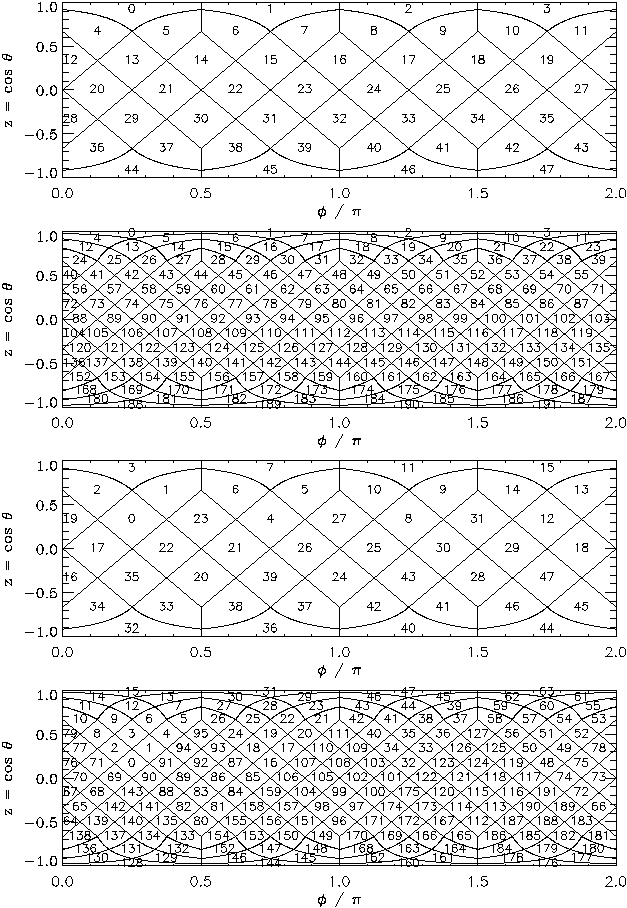
The RING and NESTED indexing schemes of HEALPix. Reproduced from The image below, reproduced from [2].
There is a third HEALPix indexing scheme called UNIQ. The UNIQ indexing scheme is special because it encodes both the resolution and the sky position in a single integer. It assigns a single unique integer to every HEALPix tile at every resolution. If ipix is the pixel index in the NESTED ordering, then the unique pixel index uniq is:
The inverse is:
FITS Format for Multi-Order Sky Maps
The FITS format for LIGO/Virgo/KAGRA multi-resolution sky maps uses the UNIQ indexing scheme and is a superset of the FITS serialization for Multi-Order Coverage (MOC) maps specified by IVOA [4] as part of the Hierarchical Progressive Survey (HiPS) capability [3], notably used by Aladin for storing and display all-sky image mosaics.
Let’s download an example multi-order FITS file with curl:
$ curl -O https://emfollow.docs.ligo.org/userguide/_static/bayestar.multiorder.fits
Let’s look at the FITS header:
$ fitsheader bayestar.multiorder.fits
# HDU 0 in bayestar.multiorder.fits:
SIMPLE = T / conforms to FITS standard
BITPIX = 8 / array data type
NAXIS = 0 / number of array dimensions
EXTEND = T
# HDU 1 in bayestar.multiorder.fits:
XTENSION= 'BINTABLE' / binary table extension
BITPIX = 8 / array data type
NAXIS = 2 / number of array dimensions
NAXIS1 = 40 / length of dimension 1
NAXIS2 = 19200 / length of dimension 2
PCOUNT = 0 / number of group parameters
GCOUNT = 1 / number of groups
TFIELDS = 5 / number of table fields
TTYPE1 = 'UNIQ '
TFORM1 = 'K '
TTYPE2 = 'PROBDENSITY'
TFORM2 = 'D '
TUNIT2 = 'sr-1 '
TTYPE3 = 'DISTMU '
TFORM3 = 'D '
TUNIT3 = 'Mpc '
TTYPE4 = 'DISTSIGMA'
TFORM4 = 'D '
TUNIT4 = 'Mpc '
TTYPE5 = 'DISTNORM'
TFORM5 = 'D '
TUNIT5 = 'Mpc-2 '
PIXTYPE = 'HEALPIX ' / HEALPIX pixelisation
ORDERING= 'NUNIQ ' / Pixel ordering scheme: RING, NESTED, or NUNIQ
COORDSYS= 'C ' / Ecliptic, Galactic or Celestial (equatorial)
MOCORDER= 11 / MOC resolution (best order)
INDXSCHM= 'EXPLICIT' / Indexing: IMPLICIT or EXPLICIT
OBJECT = 'MS181101ab' / Unique identifier for this event
REFERENC= 'https://example.org/superevents/MS181101ab/view/' / URL of this event
INSTRUME= 'H1,L1,V1' / Instruments that triggered this event
DATE-OBS= '2018-11-01T22:22:46.654437' / UTC date of the observation
MJD-OBS = 58423.93248442635 / modified Julian date of the observation
DATE = '2018-11-01T22:34:49.000000' / UTC date of file creation
CREATOR = 'BAYESTAR' / Program that created this file
ORIGIN = 'LIGO/Virgo/KAGRA' / Organization responsible for this FITS file
RUNTIME = 3.24746292643249 / Runtime in seconds of the CREATOR program
DISTMEAN= 39.76999609489013 / Posterior mean distance (Mpc)
DISTSTD = 8.308435058808886 / Posterior standard deviation of distance (Mpc)
LOGBCI = 13.64819688928804 / Log Bayes factor: coherent vs. incoherent
LOGBSN = 261.0250944470225 / Log Bayes factor: signal vs. noise
VCSVERS = 'ligo.skymap 0.1.8' / Software version
VCSREV = 'becb07110491d799b753858845b5c24c82705404' / Software revision (Git)
DATE-BLD= '2019-07-25T22:36:58' / Software build date
HISTORY
HISTORY Generated by calling the following Python function:
HISTORY ligo.skymap.bayestar.localize(event=..., waveform='o2-uberbank', f_low=3
HISTORY 0, min_inclination=0.0, max_inclination=1.5707963267948966, min_distance
HISTORY =None, max_distance=None, prior_distance_power=2, cosmology=False, mcmc=
HISTORY False, chain_dump=None, enable_snr_series=True, f_high_truncate=0.95)
HISTORY
HISTORY This was the command line that started the program:
HISTORY bayestar-localize-lvalert -N G298107 -o bayestar.multiorder.fits
This should look very similar to the FITS header for the standard HEALPix file from the previous section. The key differences are:
The
ORDERINGkey has changed fromNESTEDtoNUNIQ.The
INDXSCHMkey has changed fromIMPLICITtoEXPLICIT.There is an extra column,
UNIQ, that explicitly identifies each pixel in the UNIQ indexing scheme.The
PROBcolumn has been renamed toPROBDENSITY, and the units have change from probability to probability per steradian.
Reading Multi-Resolution Sky Maps
Now let’s go through some of the same common HEALPix operations from the previous section, but using the multi-resolution format. Instead of Healpy, we will use astropy-healpix because it has basic support for the UNIQ indexing scheme.
First, we need the following imports:
>>> from astropy.table import Table
>>> from astropy import units as u
>>> import astropy_healpix as ah
>>> import numpy as np
Next, let’s read the sky map. Instead of a special-purpose HEALPix method, we just read the FITS file into an Astropy table using Astropy’s unified file read/write interface:
>>> skymap = Table.read('bayestar.multiorder.fits')
Most Probable Sky Location
Next, let’s find the highest probability density sky position. This is a three-step process.
Find the UNIQ pixel index of the highest probability density tile:
>>> i = np.argmax(skymap['PROBDENSITY']) >>> uniq = skymap[i]['UNIQ']
What is the probability density per square degree in that tile?
>>> skymap[i]['PROBDENSITY'] * (np.pi / 180)**2 0.0782516470191411
Unpack the UNIQ pixel index into the resolution,
nside, and the NESTED pixel index,ipix, using the methodastropy_healpix.uniq_to_level_ipix(). (Note that this method returnslevel, which is the logarithm base 2 ofnside, so we must also convert fromleveltonsideusingastropy_healpix.level_to_nside().)>>> level, ipix = ah.uniq_to_level_ipix(uniq) >>> nside = ah.level_to_nside(level)
Convert from
nsideandipixto right ascension and declination usingastropy_healpix.healpix_to_lonlat()(which is equivalent tohp.pix2ang):>>> ra, dec = ah.healpix_to_lonlat(ipix, nside, order='nested') >>> ra.deg 194.30419921874997 >>> dec.deg -17.856895095545468
Probability Density at a Known Position
Now let’s look up the probability density at a known sky position. In this case, let’s use the position of NGC 4993:
>>> ra = 197.4133 * u.deg
>>> dec = -23.3996 * u.deg
Brute Force Linear Search
The following brute force method of looking up a pixel by sky position has a complexity of \(O(N)\), where \(N\) is the number of multi-resolution pixels.
Unpack the UNIQ pixel indices into their resolution and their NESTED pixel index.
>>> level, ipix = ah.uniq_to_level_ipix(skymap['UNIQ']) >>> nside = ah.level_to_nside(level)
Determine the NESTED pixel index of the target sky position at the resolution of each multi-resolution tile.
>>> match_ipix = ah.lonlat_to_healpix(ra, dec, nside, order='nested')
Find the multi-resolution tile whose NESTED pixel index equals the target pixel index.
>>> i = np.flatnonzero(ipix == match_ipix)[0] >>> i 13484
That pixel contains the target sky position.
>>> skymap[i]['PROBDENSITY'] * (np.pi / 180)**2 0.03467919098907807
Fast Binary Search
The following binary search method of looking up a pixel by sky position exploits the algebraic properties of HEALPix. It has a complexity of \(O(\log N)\) where \(N\) is the number of multi-resolution pixels. It assumes that every sky position is mapped on to exactly one multi-resolution tile, which is true for LIGO/Virgo/KAGRA multi-resolution sky maps.
First, find the NESTED pixel index of every multi-resolution tile, at an arbitrarily high resolution. (
nside = 2**29works nicely because it is the highest possible HEALPix resolution that can be represented in a 64-bit signed integer.)>>> max_level = 29 >>> max_nside = ah.level_to_nside(max_level) >>> level, ipix = ah.uniq_to_level_ipix(skymap['UNIQ']) >>> index = ipix * (2**(max_level - level))**2
Sort the pixels by this value.
>>> sorter = np.argsort(index)
Determine the NESTED pixel index of the target sky location at that resolution.
>>> match_ipix = ah.lonlat_to_healpix(ra, dec, max_nside, order='nested')
Do a binary search for that value.
>>> i = sorter[np.searchsorted(index, match_ipix, side='right', sorter=sorter) - 1] >>> i 13484
That pixel contains the target sky position.
>>> skymap[i]['PROBDENSITY'] * (np.pi / 180)**2 0.03467919098907807
Working with Flat Resolution Sky Maps
For all events, LIGO/Virgo/KAGRA also distribute the standard HEALPix
format with the file extension .fits.gz, that was the default format during
the O3 run. They are FITS image files and can be manipulated and viewed with many
commonplace FITS tools. However, they are a little unusual in two regards.
First, since they are all-sky images, they are stored in the HEALPix
[1] projection, a format that is used for Planck all-sky CMB
maps and by Aladin for hierarchical, progressively refined, all-sky survey
images (HiPS). Second, the value stored at each pixel is the probability that
the gravitational-wave source is within that pixel.
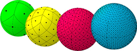
An illustration of the first four HEALPix tesselations (nside=1,
nside=2, nside=4, and nside=8). Reproduced from
https://healpix.jpl.nasa.gov.
Let’s download an example FITS file with curl:
$ curl -O https://emfollow.docs.ligo.org/userguide/_static/bayestar.fits.gz,0
We can look at the metadata inside the FITS file by printing its header with
tools like funhead from Funtools, imhead from WCSTools, or
fitsheader from Astropy:
$ fitsheader bayestar.fits.gz,0
# HDU 0 in bayestar.fits.gz,0:
SIMPLE = T / conforms to FITS standard
BITPIX = 8 / array data type
NAXIS = 0 / number of array dimensions
EXTEND = T
# HDU 1 in bayestar.fits.gz,0:
XTENSION= 'BINTABLE' / binary table extension
BITPIX = 8 / array data type
NAXIS = 2 / number of array dimensions
NAXIS1 = 32 / length of dimension 1
NAXIS2 = 50331648 / length of dimension 2
PCOUNT = 0 / number of group parameters
GCOUNT = 1 / number of groups
TFIELDS = 4 / number of table fields
TTYPE1 = 'PROB '
TFORM1 = 'D '
TUNIT1 = 'pix-1 '
TTYPE2 = 'DISTMU '
TFORM2 = 'D '
TUNIT2 = 'Mpc '
TTYPE3 = 'DISTSIGMA'
TFORM3 = 'D '
TUNIT3 = 'Mpc '
TTYPE4 = 'DISTNORM'
TFORM4 = 'D '
TUNIT4 = 'Mpc-2 '
PIXTYPE = 'HEALPIX ' / HEALPIX pixelisation
ORDERING= 'NESTED ' / Pixel ordering scheme: RING, NESTED, or NUNIQ
COORDSYS= 'C ' / Ecliptic, Galactic or Celestial (equatorial)
NSIDE = 2048 / Resolution parameter of HEALPIX
INDXSCHM= 'IMPLICIT' / Indexing: IMPLICIT or EXPLICIT
OBJECT = 'MS181101ab' / Unique identifier for this event
REFERENC= 'https://example.org/superevents/MS181101ab/view/' / URL of this event
INSTRUME= 'H1,L1,V1' / Instruments that triggered this event
DATE-OBS= '2018-11-01T22:22:46.654437' / UTC date of the observation
MJD-OBS = 58423.93248442613 / modified Julian date of the observation
DATE = '2018-11-01T22:34:49.000000' / UTC date of file creation
CREATOR = 'BAYESTAR' / Program that created this file
ORIGIN = 'LIGO/Virgo/KAGRA' / Organization responsible for this FITS file
RUNTIME = 3.24746292643249 / Runtime in seconds of the CREATOR program
DISTMEAN= 39.76999609489013 / Posterior mean distance (Mpc)
DISTSTD = 8.308435058808886 / Posterior standard deviation of distance (Mpc)
LOGBCI = 13.64819688928804 / Log Bayes factor: coherent vs. incoherent
LOGBSN = 261.0250944470225 / Log Bayes factor: signal vs. noise
VCSVERS = 'ligo.skymap 0.1.8' / Software version
VCSREV = 'becb07110491d799b753858845b5c24c82705404' / Software revision (Git)
DATE-BLD= '2019-07-25T22:36:58' / Software build date
HISTORY
HISTORY Generated by calling the following Python function:
HISTORY ligo.skymap.bayestar.localize(event=..., waveform='o2-uberbank', f_low=3
HISTORY 0, min_inclination=0.0, max_inclination=1.5707963267948966, min_distance
HISTORY =None, max_distance=None, prior_distance_power=2, cosmology=False, mcmc=
HISTORY False, chain_dump=None, enable_snr_series=True, f_high_truncate=0.95)
HISTORY
HISTORY This was the command line that started the program:
HISTORY bayestar-localize-lvalert -N G298107 -o bayestar.multiorder.fits
There are several useful pieces of information here:
COORDSYS=C, telling you that the HEALPix projection is in the Celestial (equatorial, ICRS) frame, as all LIGO/Virgo/KAGRA probability sky maps will be.OBJECT, the unique LIGO/Virgo/KAGRA identifier for the event.REFERENC, a link to the candidate page in GraceDB.INSTRUME, a list of gravitational-wave sites that triggered on the event: H1 for LIGO Hanford, L1 for LIGO Livingston, V1 for Virgo, and K1 for KAGRA.DATE-OBS, the UTC time of the event. In the case of a compact binary coalescence candidate, this is the time that the signal from the merger passed through the geocenter.MJD-OBS, same as DATE-OBS, but given as a modified Julian day.
You can view the sky map in many common FITS image viewers such as Aladin:

or DS9 (although DS9 shows HEALPix sky maps in an unusual orientation; see Figure 4 of [2] for more information.

Now, let’s go through some examples of manipulating HEALPix sky maps programmatically. The HEALPix project provides official libraries for many languages, including C, C++, Fortran, IDL, and Java. However, since this is a Python tutorial, we are going to demonstrate how to manipulate HEALPix maps with the official Python library, Healpy.
Reading Sky Maps
First, if you have not already downloaded an example sky map, you can do so now by having Python call curl on the command line:
$ curl -O https://emfollow.docs.ligo.org/userguide/_static/bayestar.fits.gz,0
Next, we need to read in the file in Python with Healpy:
>>> import healpy as hp
>>> import numpy as np
>>> hpx = hp.read_map('bayestar.fits.gz,0')
You can read both the HEALPix image data and the FITS header by passing the
h=True keyword argument:
>>> hpx, header = hp.read_map('bayestar.fits.gz,0', h=True)
Manipulating HEALPix Coordinates
The image data is a 1D array of values:
>>> hpx
array([2.70726059e-66, 1.27374324e-66, 2.62611513e-67, ...,
2.04700874e-40, 1.05781210e-35, 4.44174764e-31])
Healpy has several useful plotting routines
including hp.mollview for plotting a
Mollweide-projection all-sky map:
>>> hp.mollview(hpx)

Each entry in the array represents the probability contained within a quadrilateral pixel whose position on the sky is uniquely specified by the index in the array and the array’s length. Because HEALPix pixels are equal area, we can find the number of pixels per square degree just from the length of the HEALPix array:
>>> npix = len(hpx)
>>> sky_area = 4 * 180**2 / np.pi
>>> sky_area / npix
0.0008196227004015301
The function hp.pix2ang converts from pixel
index to spherical polar coordinates; the function hp.ang2pix does the reverse.
Both hp.pix2ang and hp.ang2pix take, as their first argument, nside, the
lateral resolution of the HEALPix map. You can find nside from the length
of the image array by calling hp.npix2nside:
>>> nside = hp.npix2nside(npix)
>>> nside
2048
Let’s look up the right ascension and declination of pixel number 123. We’ll
call hp.pix2ang to get the spherical polar
coordinates \((\theta, \phi)\) in radians, and then use np.rad2deg to convert these to right ascension and declination in degrees.
>>> ipix = 123
>>> theta, phi = hp.pix2ang(nside, ipix)
>>> ra = np.rad2deg(phi)
>>> dec = np.rad2deg(0.5 * np.pi - theta)
>>> ra, dec
(129.375, 89.81725848475484)
Let’s find which pixel contains the point RA=194.95, Dec=27.98.
>>> ra = 194.95
>>> dec = 27.98
>>> theta = 0.5 * np.pi - np.deg2rad(dec)
>>> phi = np.deg2rad(ra)
>>> ipix = hp.ang2pix(nside, theta, phi)
>>> ipix
13361492
Test if a Sky Location is in the 90% Credible Region
You can easily test if a given sky position is in the 90% credible region. Let’s continue using the sky position from the previous example, for which we have already determined the pixel index.
Use the following simple algorithm to construct a map that gives the credible level of each pixel:
Sort the pixels by descending probability density.
Cumulatively sum the pixels’ probability.
Return the pixels to their original order.
In Python, you can use this simple recipe:
>>> i = np.flipud(np.argsort(hpx))
>>> sorted_credible_levels = np.cumsum(hpx[i])
>>> credible_levels = np.empty_like(sorted_credible_levels)
>>> credible_levels[i] = sorted_credible_levels
>>> credible_levels
array([1., 1., 1., ..., 1., 1., 1.])
Note
Observe that the values in the resulting credible level map vary inversely with probability density: the most probable pixel is assigned to the credible level 0.0, and the least likely pixel is assigned the credible level 1.0.
Tip
This recipe is implemented in the package
ligo.skymap as the function
find_greedy_credible_levels():
>>> from ligo.skymap.postprocess import find_greedy_credible_levels
>>> credible_levels = find_greedy_credible_levels(hpx)
>>> credible_levels
array([1., 1., 1., ..., 1., 1., 1.])
To check if the pixel that we identified in the previous section is within the 90% credible level, simply test if the value of the credible level map is less than or equal to 0.9 at that pixel:
>>> credible_levels[ipix]
0.9999999999947833
>>> credible_levels[ipix] <= 0.9
False
The credible level map has a value greater than 0.9 at that sky location, therefore the sky location is outside the 90% credible region.
Find the Area of the 90% Credible Region
Since we just found the credible level map, it’s easy to compute the 90% credible area by counting the number of pixels inside the 90% credible region and multiplying by the area per pixel.
In the Python expression below, note that (credible_levels <= 0.9)
evaluates to a binary array; when it is summed over, true values are treated as
1 and false values are treated as 0.
>>> np.sum(credible_levels <= 0.9) * hp.nside2pixarea(nside, degrees=True)
30.979279207076633
Most Probable Sky Location
Let’s find the highest probability pixel.
>>> ipix_max = np.argmax(hpx)
What is the probability density per square degree at that position?
>>> hpx[ipix_max] / hp.nside2pixarea(nside, degrees=True)
0.0782516470191411
Where is the highest probability pixel on the sky? Use hp.pix2ang.
>>> theta, phi = hp.pix2ang(nside, ipix_max)
>>> ra = np.rad2deg(phi)
>>> dec = np.rad2deg(0.5 * np.pi - theta)
>>> ra, dec
(194.30419921875, -17.856895095545475)
Integrated Probability in a Circle
How do we find the probability that the source is contained within a circle on
the sky? First we find the pixels that are contained within the circle using
hp.query_disc. Note that this function takes as its
arguments the Cartesian coordinates of the center of the circle, and its radius
in radians. Then, we sum the values of the HEALPix image array contained at
those pixels.
First, we define the RA, Dec, and radius of circle in degrees:
>>> ra = 213.22
>>> dec = -37.45
>>> radius = 3.1
Then we convert to spherical polar coordinates and radius of circle in radians:
>>> theta = 0.5 * np.pi - np.deg2rad(dec)
>>> phi = np.deg2rad(ra)
>>> radius = np.deg2rad(radius)
Then we calculate the Cartesian coordinates of the center of circle:
>>> xyz = hp.ang2vec(theta, phi)
We call hp.query_disc, which returns an array of
the indices of the pixels that are inside the circle:
>>> ipix_disc = hp.query_disc(nside, xyz, radius)
Finally, we sum the probability in all of the matching pixels:
>>> hpx[ipix_disc].sum()
3.655661941088471e-10
Integrated Probability in a Polygon
Similarly, we can use the hp.query_polygon
function to look up the indices of the pixels within a polygon (defined by the
Cartesian coordinates of its vertices), and then compute the probability that
the source is inside that polygon by summing the values of the pixels.
>>> xyz = [[-0.69601758, -0.41315628, -0.58724902],
... [-0.68590811, -0.40679797, -0.60336181],
... [-0.69106913, -0.39820114, -0.60320752],
... [-0.7011786 , -0.40455945, -0.58709473]]
>>> ipix_poly = hp.query_polygon(nside, xyz)
>>> hpx[ipix_poly].sum()
1.128695302404769e-12
These are all of the HEALPix functions from Healpy that we will need for the remainder of the this tutorial.
Other useful Healpy functions include hp.ud_grade for upsampling or downsampling a sky map and
hp.get_interp_val for performing
bilinear interpolation between pixels. See the Healpy tutorial for other useful operations.
Basic Observability Calculations
Now we are going to teach our GCN handler how to determine whether a gravitational-wave event is observable. We are going to use the astropy.coordinates module. (See also the Astropy example on observation planning in Python.) First, we will need to import a few extra Python modules:
import astropy.coordinates
import astropy.time
import astropy.units as u
The LIGO/Virgo/KAGRA probability sky maps are always in equatorial coordinates. Once we have looked up the coordinates of the HEALPix pixels, we will use Astropy to transform those coordinates to a horizontal (altitude–azimuth) frame for a particular site on the Earth at a particular time. Then we can quickly determine which pixels are visible from that site at that time, and integrate (sum) the probability contained in those pixels.
Note
You may want to do something more sophisticated like determine how much of
the probability is visible for at least a certain length of time. This
example will illustrate one key function of HEALPix (looking up coordinates
of the grid with hp.pix2ang) and some of
the key positional astronomy functions with Astropy. For more advanced
functionality, we recommend the astroplan package.
def prob_observable(m, header):
"""
Determine the integrated probability contained in a gravitational-wave
sky map that is observable from a particular ground-based site at a
particular time.
Bonus: make a plot of probability versus UTC time!
"""
# Determine resolution of sky map
npix = len(m)
nside = hp.npix2nside(npix)
# Get time now
time = astropy.time.Time.now()
# Or at the time of the gravitational-wave event...
# time = astropy.time.Time(header['MJD-OBS'], format='mjd')
# Or at a particular time...
# time = astropy.time.Time('2015-03-01 13:55:27')
# Geodetic coordinates of observatory (example here: Mount Wilson)
observatory = astropy.coordinates.EarthLocation(
lat=34.2247*u.deg, lon=-118.0572*u.deg, height=1742*u.m)
# Alt/az reference frame at observatory, now
frame = astropy.coordinates.AltAz(obstime=time, location=observatory)
# Look up (celestial) spherical polar coordinates of HEALPix grid.
theta, phi = hp.pix2ang(nside, np.arange(npix))
# Convert to RA, Dec.
radecs = astropy.coordinates.SkyCoord(
ra=phi*u.rad, dec=(0.5*np.pi - theta)*u.rad)
# Transform grid to alt/az coordinates at observatory, now
altaz = radecs.transform_to(frame)
# Where is the sun, now?
sun_altaz = astropy.coordinates.get_sun(time).transform_to(altaz)
# How likely is it that the (true, unknown) location of the source
# is within the area that is visible, now? Demand that sun is at
# least 18 degrees below the horizon and that the airmass
# (secant of zenith angle approximation) is at most 2.5.
prob = m[(sun_altaz.alt <= -18*u.deg) & (altaz.secz <= 2.5)].sum()
# Done!
return prob
Finally, we need to update our GCN handler to call this function:
@gcn.handlers.include_notice_types(
gcn.notice_types.LVC_PRELIMINARY,
gcn.notice_types.LVC_INITIAL,
gcn.notice_types.LVC_UPDATE)
def process_gcn(payload, root):
# Respond only to 'test' events.
# VERY IMPORTANT! Replce with the following line of code
# to respond to only real 'observation' events.
# if root.attrib['role'] != 'observation':
# return
if root.attrib['role'] != 'test':
return
# Respond only to 'CBC' events. Change 'CBC' to "Burst'
# to respond to only unmodeled burst events.
if root.find(".//Param[@name='Group']").attrib['value'] != 'CBC':
return
skymap_url = root.find(".//Param[@name='skymap_fits']").attrib['value']
skymap, header = hp.read_map(skymap_url, h=True)
prob = prob_observable(skymap, header)
print('Source has a {:d}% chance of being observable now'.format(
int(round(100 * prob))))
if prob > 0.5:
pass # FIXME: perform some action
Let’s run the new GCN handler now…
# Listen for GCNs until the program is interrupted
# (killed or interrupted with control-C).
gcn.listen(handler=process_gcn)
When you run this script, each time you receive a sample LIGO/Virgo/KAGRA GCN Notice, it will print something like the following (note that probability will change as a function of time):
Source has a 76% chance of being observable now
Distance and 3D Sky Maps
All sky localization FITS files for CBC events are three dimensional: they include both the sky probability map and a directionally dependent distance estimate. This can be useful for identifying possible host galaxies using a galaxy redshift catalog. For further details see [1] and for sample code see [2].
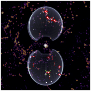
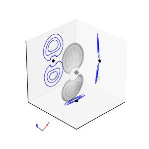
Additional Resources
Here are a few additional resources for working with LIGO/Virgo/KAGRA alerts.
ligo.skymap: Advanced Python Tools for Probability Sky Maps
The ligo.skymap Python package includes a number of advanced tools for working with GW probability sky maps.
Publication-quality astronomical mapmaking built on Astropy (
ligo.skymap.plot.allsky)
Functions for manipulating distance posteriors (
ligo.skymap.distance)Probabilistic airmass plots (ligo-skymap-plot-airmass)
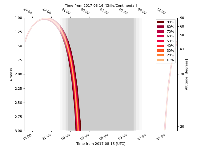
The rapid sky localization code BAYESTAR, which is used to produce the initial sky maps for CBC events but can also be used to create simulated sky localizations.
The postprocessing tool that creates updated sky maps from MCMC samples (ligo-skymap-from-samples)
Sky Map Visualizations and Credible Regions in Aladin
In this section, we demonstrate working with gravitational-wave sky localizations in Aladin Desktop. The following main topics are addressed.
MOC and GW Sky Localizations
The enclosed area within a given probability level contour of a GW sky map can be effectively described with a Multi-Order Coverage (MOC) map [1]. MOC is a standard of the Virtual Observatory which provides a representation of arbitrary regions on the unit sphere using the HEALPix sky tessellation.
The MOC data structure encodes irregular sky regions as a hierarchy of HEALPix
pixels. Each MOC cell is defined by two numbers: the hierarchy level (HEALPix
\(\mathit{order}\)) and the pixel index (HEALPix \(\mathit{ipix}\)).
MOCs are serialized as FITS or JSON files. The finest level of refinement
within the MOC hierarchy is determined by the HEALPix \(\mathit{order}\)
parameter or the equivalent \(\mathit{nside}\) parameter, related by
\(\mathit{nside} = 2^\mathit{order}\). For example, order=9 corresponds
to nside=512, and a resolution of \(6.9'\) per pixel.
The MOC maps make database queries for retrieving objects and logical operation (such as union, intersection, subtraction, difference) extremely fast even for very complex sky regions.
MOC maps and multi-order sky maps are closely related. They use similar multi-resolution HEALPix data structures. The main distinction is that MOC maps encode regions on the sphere, whereas multi-order sky maps encode sampled images or functions on the sphere. The multi-order sky map FITS format is a superset of the MOC FITS format, the only difference being that a multi-order sky map has values attached to each cell (probability density, distance estimates) whereas a MOC map does not. Aladin version v12 supports the LIGO/Virgo/KAGRA multi-resolution sky maps.
Running Aladin Desktop
Aladin Desktop is a Java application. To run it, you must first have the Java Virtual Machine (JVM) installed. More details are in Aladin’s download page.
Note
Aladin may fail to load some LIGO/Virgo/KAGRA sky maps and display a
java.lang.OutOfMemoryError error message. This is because the highest
resolution LIGO/Virgo/KAGRA sky maps do not fit inside Aladin’s default
memory size.
You can increase the maximum memory size used by your Java runtime environment by following the instructions below.
Download the Aladin.jar from the Aladin download page. Execute it from a terminal by typing:
$ java -Xmx2g -jar Aladin.jar
The flag -Xmx<ammount of memory> specifies the maximum memory
allocation pool for a JVM. Here 2GB of memory is allocated. For GW sky
localizations with nside=2048, increase the memory allocated up to 3GB,
-Xmx3g.
Loading a GW Sky Localization
You can copy and paste the sky map URL from the GraceDB or drag and drop a
HEALPix FITS file from your operating system’s file browser in the main Aladin
window. Aladin v12 recognizes both the standard HEALPix format with the file
extension .fits.gz and the multi-resolution HEALPix format, distinguished
by the file extension .multiorder.fits. Better performances are achieved with
the multi-resolution format. Here we will work with the LALInference sky map of
GW170817.
Building a Credible Region
The sequence of the Aladin Desktop commands to create a credible region at a defined confidence level is described below. From the menu bar, select .

The MOC generation window has three options: the probability sky map, the threshold, and the MOC resolution. Make sure that the GW sky map that we loaded in the previous step is selected in the Proba skymap dropdown menu. Then enter a number between 0 and 1 for the credible level in the Probability threshold box. Finally, press the CREATE button. The MOC for the credible region is created and loaded in the Aladin Stack. If you repeat this process multiple times for different credible levels, then you can select each MOC independently from the Aladin stack.
Area Within a Credible Region
There are two ways to get the area within a MOC credible region. If you hover over the cursor over the MOC name in the Aladin stack, then the area in square degrees and the percentage of the sky are shown in the top-right corner of the Aladin window. Alternatively, you can right-click the MOC in the Aladin stack and select Properties from the contextual menu. The area and percentage of the sky are shown in the Properties dialog box. From this dialog box, you can also control the appearance and color of the MOC, which is useful for distinguishing multiple MOCs for different credible levels.

Querying and Filtering a Galaxy Catalog
Each gravitational-wave sky map for a CBC event provides a three-dimensional probability distribution as a function of sky position and distance [2]. Cross-matching that distribution with positions and redshifts of a galaxy catalog provides a filtered list of of possible host galaxies (see Distance and 3D Sky Maps). Aladin does not yet implement a galaxy catalog query by the three-dimensional posterior probability distribution. However, it is currently possible in Aladin to search for galaxies within the 2D credible region on the sky and, afterwards, apply a distance cut that it independent of sky position.
Here we query the galaxies collected in the GLADE catalog inside the 90% credible region of GW170817. Then we filter those galaxies according to the marginal distance posterior distribution integrated over the whole sky.
Pick out the galaxy catalog from the data collections tree.
Any of the 20,000 catalogs published in the Virtual Observatory can be retrieved from the data collections tree in the left panel of the main Aladin window.
To find the GLADE catalog, make sure that is selected in the from dropdown menu in the bottom of the left panel, then type
GLADEin the select text field. In the data collections tree, click on .Load the galaxy catalog filtered by the 2D credible region.
In the popup window, click the by region & MOC checkbox in order to filter it by the 2D credible region that we created earlier. Then press the Load button.

Filter the galaxy catalog by distance.
The posterior mean distance and the posterior standard deviation of luminosity distance in Mpc are reported in the FITS file header with the keywords
DISTMEANandDISTSTD, respectively. In the case of GW170817, they have the valuesDISTMEAN = 38.0andDISTSTD = 7.5.Select from the menu bar. This opens the Properties dialog box contains two tabs. Select the Advanced mode tab and copy the following text into the filter definition box:
${Dist} > 30.5 && ${Dist} < 45.5 {draw}This is an expression for a 1-sigma cut on distance in the Aladin filter syntax.
Distis the column in the GLADE catalog corresponding to the distance in Mpc.Click on Apply and then on Export to create a new level in the Aladin stack consisting only of sources selected by the filter.

Thumbnail View Generator
Finally, we make a mosaic of the filtered galaxies. Here the thumbnails are color composition images of the Digitized Sky Surveys (DSS).

To get this, we load the DSS colored survey from the data collections tree. Then select from the menu bar, and click the Ok button in the dialog box. Aladin will generate thumbnail views from the current image in the main window. To change it, check the corresponding plan in the Aladin stack.
Building a Spatial and Temporal Credible Region
Aladin v12 offers the functionality to add temporal information in any spatial coverage described by the MOC data structure. The resulting new data structure is indicated with STMOC (Space and Time MOC) [3].
Click on the name of the plan corresponding to the credible region.
MOC 0.9 GW170817_skymap.fits will appear highlighted.
From the menu bar, press
.
The Properties is equipped with the Time section with
two boxes in which you can select a time interval.
The merge time of GW170817 occurs at 2017-08-17T12:41:04.43 UTC.
Searching for coincident with external triggers, we apply a time window
from -1 s to 5 s around the GW time i.e., from
2017-08-17T12:41:03.43 UTC to 2017-08-17T12:41:09.43 UTC.
Click on Apply to create a credible region with this time range. The main Aladin window shows a bottom box Time plot displaying the associated time line.

Spatial and Temporal Coverage Intersections
The STMOC data structure allows you to perform operations in space and time simultaneously. We build a new STMOC with the error box of GRB 170817 provided by the GBM instrument on board the Fermi satellite. GRB170817 occurred at 2017-08-17T12:41:06 UTC [4].
The intersection is performed by opening the window Logical operations from . An additional MOC layer is loaded into the Aladin stack with information on the spatial and temporal coincident of the two astrophysical events.

Mobile Apps
There are two unofficial apps for mobile devices. Install one of these apps to view GW alerts on your smart phone or tablet.
Gravitational Wave Events for iOS by Peter Kramer
Gravitational Wave Treasure Map
This webpage is helpful for astronomers in coordinating electromagnetic follow-up of gravitational-wave events.
✨Early-Warning Alerts
BNS mergers spend several minutes in band of the Advanced ground-based gravitational-wave detectors. For some loud and nearby BNS mergers, it is possible to accumulate enough SNR and detect them several tens of seconds before merger. During O3, automated public alerts for CBC events have been sent within as little as 2 minutes after merger. In O4, we will be deploying search pipelines that can in principle detect BNS events before merger.
Since it is generally assumed that detectable electromagnetic (or neutrino) emission starts shortly after merger, a pre-merger gravitational-wave detection would provide early warning of an impending electromagnetic transient and might make it possible for automated follow-up facilities to capture any prompt emission from the merger environment, the jet, and other unknown activity.
We had previously conducted a trial early warning public alert infrastructure in June 2020 replaying an 8-day period of archival LIGO data from O3. Results from this study were published in [1]. This study demonstrated that in principle it is possible to sent out GCN Notices in advance of a BNS merger. Based on the current expect BNS merger rate, we expect O(1) event per year to be detected before merger in O4.
We have commissioned capability to produce and distribute early warning gravitational-wave alerts up to tens of seconds before merger. We have also reduced the latency of ordinary post-merger alerts to within tens of seconds after merger.
Subscribe to Early-Warning Alerts
Early warning alerts are publicly distributed as Notices just like ordinary gravitational-wave alerts (see the Alert Contents section). They have exactly the same format and content as a Preliminary Notice. In particular, early warning GCN Notices have significance estimates, sky localizations, and source classifications. Also, like Preliminary GCN Notices, Early Warning Notices are sent prior to vetting by humans, and are not accompanied by a GCN Circular.
Early warning GCN Notices are differentiated from ordinary GCN Notices by the
new LVC_EARLY_WARNING GCN Notice type. If you are receiving GCN Notices via
an anonymous VOEvent connection and you are using the Python sample code from
the VOEvent Notices via GCN Classic section, then all you have to do is add
the notice type to your GCN handler:
import gcn
@gcn.handlers.include_notice_types(
gcn.notice_types.LVC_EARLY_WARNING, # <-- new notice type here
gcn.notice_types.LVC_PRELIMINARY,
gcn.notice_types.LVC_INITIAL,
gcn.notice_types.LVC_UPDATE,
gcn.notice_types.LVC_RETRACTION)
def process_gcn(payload, root):
... # <-- put your code here
gcn.listen(handler=process_gcn)
(If you are using a non-anonymous GCN connection or one of the many other notice formats provided by GCN, then you will also need to submit a change to your GCN Notice subscription settings.)
Important
Since these early-warning events will arise from time-shifted and replayed
data and not live observations, the GCN notices will be flagged as test
events by setting the VOEvent role="test" attribute.
Detection Method
All of our CBC search pipelines (GstLAL [2], MBTA, PyCBC, and SPIIR) are participating in early-warning alerts. See the Online Pipelines section for details on these analyses. Localizations will be produced with BAYESTAR; see the Sky Localization and Parameter Estimation section for details.
BNS signals sweep up smoothly in frequency for a few minutes across the Advanced LIGO band. In that time, they may accumulate enough SNR to be detected before merger. A GW170817-like system with a total network SNR of 32 will already accumulate an SNR of 11 by the time the signal sweeps up to 30 Hz, about a minute before merger.

The time evolution of the gravitational-wave frequency and the cumulative SNR for a GW170817-like BNS system.
The early warning search is a matched-filter search that uses templates that have been truncated at a selection of end frequencies—or equivalently, cut off at a selection of times before merger.
Source Classification
The automated source classification and properties have not been trained or tested extensively for early warning alerts. However, the early warning analysis is only sensitive to BNS-mass mergers. As a result, the favored source class in early warning GCN Notices will always be either BNS or Terrestrial, with a 0% chance of NSBH or BBH. The HasNS and HasRemnant fields will always show 100%.
Localization
Sky localizations for early warning alerts are typically very coarse because the early warning analysis inherently does not make use of the full duration and bandwidth of the gravitational-wave signal. The localization improves slowly up until the last second before merger, and then converges rapidly in the last second.
The animations below taken from the data release [3] show the evolution of early-warning sky maps for three representative events with different SNR values. Note that this study assumed the detectors to be operating at their final design sensitivity.
Final SNR |
11 |
18 |
25 |
|---|---|---|---|
Distance |
250 Mpc |
210 Mpc |
160 Mpc |
Sky map (animated GIF) |
|
|
|
Frequency |
Localization accuracy (90% credible area) |
||
29 Hz |
Not detected |
Not detected |
12000 deg2 |
32 Hz |
10000 deg2 |
||
38 Hz |
9200 deg2 |
8200 deg2 |
|
49 Hz |
2300 deg2 |
1000 deg2 |
730 deg2 |
56 Hz |
1000 deg2 |
700 deg2 |
250 deg2 |
1024 Hz |
10 deg2 |
31 deg2 |
5.4 deg2 |
Appendix
Change Log
Version 17.1 (2022-12-14)
Sample Code
Fix a copy-paste error in the GCN sample code.
Version 17 (2022-12-14)
General
Change the name of this document from “LIGO/Virgo Public Alerts User Guide” to “LIGO/Virgo/KAGRA Public Alerts User Guide”.
Use the new sphinx-immaterial-igwn theme which is common to many LIGO/Virgo/KAGRA documents.
Multi-resolution FITS files are now the preferred format for sky maps.
Add tutorial on receiving and parsing notices distributed over Kafka via GCN and SCiMMA. This change is reflected in multiple sections: Alert Contents and Sample Code.
Remove
MassGapfrom source classification and addHasMassGapto source properties. This change is reflected in multiple sections: Data Analysis, Alert Contents, and Sample Code.
Observing Capabilities
Update the observing timeline, detection and localization estimates, and sample sky maps data release for O4 and O5.
Data Analysis
Several changes to source properties:
Add a reference to the source properties methods paper.
Add details on equation of state marginalization.
Alert Contents
Add RAVEN space-time coincidence FAR to alert example.
Add INTEGRAL to notice types considered by RAVEN.
Add a terminal
Zto all time strings in the VOEvents to that they are in the UTC time zone and to conform to the ISO 8601 date-time format. See RFC 3339.
Sample Code
Update information on working on multi-resolution sky maps. Changed the presentation order to reflect that multi-resolution is now the default.
Additional Resources
Update information about early warning, pre-merger for compact binary events.
Add a link to the Gravitational Wave Treasure Map.
Version 16 (2020-05-28)
General
Add the new ✨Early-Warning Alerts section to introduce early warning alerts as a public post-O3 technology demonstration. Early warning alerts are detections of binary neutron star merger candidates up to tens of seconds before merger. Starting on 2020-06-09 and lasting for one week, simulated early-warning alerts from replayed O3 LIGO/Virgo data will be publicly distributed at a rate of approximately once per day.
Observing Capabilities
Note suspension of Observing Run 3 (O3) on March 27, 2020, due to the COVID-19 pandemic. When it becomes safe to resume normal activities, there may be a short period of additional O3 observations before an extended shutdown to prepare for the next observing run (O4). Updates will be posted in this document as they become available.
Alert Contents
Add an example EarlyWarning GCN notice.
Version 15 (2020-01-15)
Observing Capabilities
Add sensitivity, detection rate, and localization accuracy statistics for O3 and O4 from the most recent arXiv submission of the LIGO/Virgo/KAGRA observing scenarios paper, arXiv:1304.0670. Add ranges for BBH and NSBH sources. Update O3 timeline and range schedule figures. Expect another update in the next few weeks incorporating O3a.
Version 14 (2020-01-06)
Data Analysis
Change FAR threshold due to the additional trials from the GRB coincidence search.
Alert Contents
Add VOEvent documentation and examples for gravitational-wave events that are coincident with GRBs.
Version 13 (2019-12-16)
Data Analysis
Add a note that the oLIB search is not currently in operation.
Alert Contents
Add a warning that VOEvent over anonymous VTP is the only GCN format and distribution method that is fully supported by LIGO/Virgo/KAGRA. In particular, LIGO/Virgo/KAGRA performs only limited quality control control checks for the textual “full format” and the binary format.
In the VOEvent alert schema, add a
nameattribute to each<Group>tag so that parameter groups are recognized by theget_grouped_params()function from the voevent-parse package. For backwards compatibility, both thenameattribute and thetypeattribute will be set to the same value.The groups are now denoted as follows:
<Group name="GW_SKYMAP" type="GW_SKYMAP">for localization parameters<Group name="Classification" type="Classification">for compact binary source classification parameters<Group name="Properties" type="Properties">for compact binary source properties parameters
Additional Resources
Add the Chirp mobile app for iOS and Android by Laser Labs.
Version 12 (2019-10-24)
Observing Capabilities
Update ranges and rates based on up-to-date O3 analysis. Add BBH and NSBH ranges. Update range and observing schedule figures.
Generalize the definition of the range so that it is unambiguous at high redshift. It is now defined as in arXiv:1709.08079.
Add the end date of Observing Run 3 (O3) on 2020-04-30.
Data Analysis
Document the false alarm rate threshold for public alerts.
Alert Contents
Remove the documentation for the Fluence parameter from burst alerts because it is not currently present in the VOEvents.
Update the list of pipeline names that can appear in GCN Notices.
Additional Resources
Created a new section for additional and contributed tools. The ligo.skymap and Aladin pages have been moved into this section.
Add instructions for cross-matching sky localizations with galaxy catalogs in Aladin Desktop.
Add the unofficial iOS Gravitational Wave Events app.
Version 11 (2019-09-15)
Data Analysis
Update the documentation about superevents describing the criteria by which the preferred event is selected. For CBC events, events with three detectors are preferred over two detectors, and events with two detectors are preferred over events with one detector.
Alert Contents
Add references to the HEALPix paper (Górski et al. 2005, doi:10.1086/427976).
Add version number suffixes to sky map FITS filenames in GCN notices to distinguish between different sky maps with the same filename. For example, the first file with the name
bayestar.fits.gzwill be referred to asbayestar.fits.gz,0, then the next will bebayestar.fits.gz,1, and so on. The filename with no version suffix always points to the most recent version.
Sample Code
Add attribution for a HEALPix illustration that was reproduced from https://healpix.jpl.nasa.gov.
Fix the example image for
hp.mollview(), which was distorted due to a file conversion issue.Add section on sky map visualization and credible regions in Aladin.
Version 10 (2019-07-31)
Data Analysis
Add a more detailed description of the RAVEN pipeline. Previously just mentioned types of searches but now has information on external experiments, coincident searches, and coincident false alarm rates.
Fixed PyCBC Live reference.
Alert Contents
Changed the data type of the
UNIQcolumn of the multi-order sky map format from an unsigned integer to a signed integer as specified by the MOC-in-FITS standard.This will improve interoperability with the mrdfits function from the IDL Astronomy User’s Library and the fv FITS Viewer from FTOOLS, both of which were reported to have problems with the old unsigned integer column. It will also make it simpler to work with Numpy indexing operations, since Numpy uses a signed integer type for indexing.
This change will go into effect in the LIGO/Virgo/KAGRA low-latency alert system on 2019-08-06.
Users of ligo.skymap should update to version 0.1.8 or newer because older versions will be unable to read old files with unsigned
UNIQcolumns. The new version ofligo.skymapcan read files with either signed or unsignedUNIQcolumns.
Version 9 (2019-06-13)
General
There is now a shorter URL for the Public Alerts User Guide, which can now be found at either https://emfollow.docs.ligo.org or https://emfollow.docs.ligo.org/userguide.
Data Analysis
Renamed this section from “Procedures” to “Data Analysis” and reordered its subsections to better reflect the chronological order of the steps of the analysis.
Sample Code
Remove MacPorts installation instructions.
Add tutorial on working with multi-resolution sky maps.
Add sample code to test whether a sky position is in the 90% credible region.
Add sample code to find the area of the 90% credible region.
Version 8 (2019-05-22)
Alert Contents
Describe the two localization formats, the official
*.fits.gzHEALPix-in-FITS format and the experimental multi-resolution HEALPix*.multiorder.fitsformat.Effective 2019-05-28, the multi-resolution file suffix will be renamed from
*.fitsto*.multiorder.fits. The old*.fitssuffix had caused confusion because the multi-resolution format is not the same as the*.fits.gzfiles without gzip compression.The multi-resolution format is currently recommended only for advanced users. Tutorials and sample code will soon be included in an upcoming version of the User Guide.
Update the description of the
HasNSproperty in the sample GCN Notices. Previously, it was defined as the probability that at least one object in the binary has a mass that is less than 2.83 solar masses. Now, for consistency with the source classification definitions, it is defined as the probability that at least one object in the binary has a mass that is less than 3 solar masses.Add some shading to the source classification diagram to make it clear that the definitions of the source classes are symmetric under exchange of the component masses, but that by convention the component masses are defined such that \(m_1 \geq m_2\).
Version 7.1 (2019-03-02)
Remove the warning on the front page about significant changes to this document occurring before the start of O3.
Version 7 (2019-03-02)
Observing Capabilities
Record the official start of O3.
Procedures
Add Gravitational Wave/High Energy Neutrino search to the list of multi-messenger search pipelines.
Sample Code
Add instructions for installing required packages using the Anaconda Python distribution.
Version 6 (2019-03-08)
Alert Contents
Switch to the GW170817 Hanford-Livingston-Virgo localization for the example sky map.
Version 5 (2019-03-01)
Alert Contents
Add a human-readable description to the
Pkt_Ser_Numparameter.Add
<EventIVORN cite="supersedes">elements to the sample Initial and Update notices in order to cite all prior VOEvents. GraceDB already includes this metadata, but it was missing from the examples.Add MassGap classification for compact binary mergers.
Version 4 (2019-02-15)
General
Changed the contact email to <emfollow-userguide@support.ligo.org> because some mail clients had trouble with the slash in the old contact email address, <contact+emfollow/userguide@support.ligo.org>. (The old address will also still work.)
Getting Started Checklist
Update links for OpenLVEM enrollment instructions.
Observing Capabilities
Update planned dates for Engineering Run 14 (ER14; starts 2019-03-04) and Observing Run 3 (O3; starts 2019-04-01).
Add Live Status section, listing some public web pages that provide real-time detector status.
Sample Code
Update the example GCN notice handler so that it does not fail if the notice is missing a sky map, because as we have specified them,
LVC_RETRACTIONnotices never contain sky maps andLVC_PRELIMINARYnotices may or may not contain sky maps.When building the documentation, test all of the sample code automatically.
Version 3 (2019-02-13)
Alert Contents
Remove the
skymap_pngparameter from the VOEVents. The sky map plots take longer to generate than the FITS files themselves, so they would have needlessly delayed the preliminary alerts.Change the IVORN prefix from
ivo://gwnet/gcn_sendertoivo://gwnet/LVC, because GCN traditionally uses the text after the/to indicate the name of the mission, which most closely corresponds to “LVC,” short for “LIGO/Virgo/KAGRA Collaboration.” Note that this IVORN is used for historical purposes and continuity with the GCN notice format used in O1 and O2, and is likely to change in the future with the commissioning of additional gravitational-wave facilities.Retraction notices now get a separate GCN notice packet type,
LVC_RETRACTION=164. TheRetractionparameter has been removed from the<What>section.
Version 2 (2018-12-13)
Alert Contents
Removed the
Vettedparameter from GCN Notices. It was intended to indicate whether the event had passed human vetting. However, it was redundant because by definition Preliminary events have not been vetted and all Initial and Update alerts have been vetted.The type of the
Retractionparameter in the GCN Notices was changed from a string (falseortrue) to an integer (0or1) for consistency with other flag-like parameters.Remove the
unitsattribute from parameters that are not numbers.
Sample Code
GCN has now begun publicly broadcasting sample LIGO/Virgo/KAGRA GCN Notices. Updated the sample code accordingly with instructions for receiving live sample notices.
Version 1 (2018-11-27)
Getting Started Checklist
Updated instructions for joining the OpenLVEM Community.
Observing Capabilities
Changed the expected number of BNS events in O3 from 1-50, as stated in the latest version of the Living Review, to 1-10 events, as stated in the more recent rates presentation.
Alert Contents
In the example VOEvents, moved the Classification and Inference quantities from the
<Why>section to the<What>section so that they validate against the VOEvent 2.0 schema.
Glossary
- Avro
Apache Avro is an open, binary data serialization format. See https://avro.apache.org for more information.
- Base64
A common binary encoding scheme supported by many open-source libraries, e.g. the python stadard library.
- BBH
Binary black hole, a binary system composed of two black holes. See BH.
- BH
Black hole.
- BNS
Binary neutron star, a binary system composed of two neutron stars. See NS.
- burst
In the context of gravitational waves, a signal candidate that is detected without a template and without prior knowledge of the waveform. Examples of potential sources of gravitational-wave bursts include high mass BBH mergers, core-collapse supernovae, and cosmic string cusps.
- chirp mass
In a binary system, the chirp mass is a symmetric combination of the primary and secondary component masses \(m_1\) and \(m_2\) that parameterizes the leading-order time or frequency evolution of the gravitational-wave signal. It is usually denoted by a script “M” symbol, \(\mathcal{M}\), and is defined as \(\mathcal{M} = (m_1 m_2)^{3/5} (m_1 + m_2)^{-1/5}\).
- CBC
Compact binary coalescence.
- EOS
Equation of state. The equation of state determines the relation between mass and radius, or mass and compactness, or pressure and (mass, energy, or number) density, of neutron stars.
- FAR
False alarm rate, a statistic that is used to describe the significance of a gravitational-wave event. See section false alarm rate (FAR) for details. FAR has units of frequency (one over time).
- FITS
Flexible Image Transport System, a format for astronomical tables, images, and multidimensional data sets. See NASA’s FITS Support Office (https://fits.gsfc.nasa.gov) for specifications, software, and documentation.
- GCN
The General Coordinates Network (https://gcn.nasa.gov), a NASA-hosted public portal for discoveries and observations of astronomical transients. GCN hosts one of the Kafka brokers used to distribute LIGO/Virgo/KAGRA alerts. See https://gcn.nasa.gov.
- GCN Circular
A human-readable astronomical bulletin distributed through GCN.
- GraceDB
Gravitational Wave Candidate Event Database (https://gracedb.ligo.org), the official public marshal portal for LIGO/Virgo/KAGRA candidates.
- GRB
Gamma-ray burst.
- HEALPix
Hierarchical Equal Area isoLatitude Pixelation, a scheme for indexing positions on the unit sphere. See https://healpix.sourceforge.io.
- HEN
High Energy Neutrino, particularly in the context of multi-messenger GW+HEN follow-up.
- JSON
JavaScript Object Notation is an open data serialization format. JSON-serialized data look like JavaScript literals. See https://json.org for more information.
- Kafka
Apache Kafka is an open-source distributed event streaming platform. See https://kafka.apache.org for more information.
- KAGRA
Kamioka Gravitational Wave Detector (see KAGRA home page), an underground gravitational-wave detector in the Kamioka mine in Japan.
- LHO
LIGO Hanford Observatory (see LHO observatory home page), site of a 4 km gravitational-wave detector in Hanford, Washington, USA.
- LLO
LIGO Livingston Observatory (see LLO observatory home page), site of a 4 km gravitational-wave detector in Livingston, Louisiana, USA.
- MassGap
Compact binary systems with at least one compact object whose mass is in the hypothetical “mass gap” between neutron stars and black holes, defined here as 3-5 solar masses.
- MCMC
Markov chain Monte Carlo. A numerical algorithm for sampling complex, multidimensional probability distributions, or for integrating functions of many variables. Used extensively in gravitational-wave parameter estimation.
- MOC
Multi-Order Coverage map, a format to describe the coverage of an arbitrary region on the unit sphere. A MOC consists of a list of HEALPix cells at different depths. For the specification, see the HiPS IVOA Recommendation.
- Notice
- NS
Neutron star.
- NSBH
Neutron star black hole, a binary system composed of one neutron star and one black hole. See NS, BH.
- O1
Advanced LIGO and Advanced Virgo’s first observing run.
- O2
Advanced LIGO and Advanced Virgo’s second observing run.
- O3
Advanced LIGO and Advanced Virgo’s third observing run.
- primary
When referring to the two component compact objects or the masses of the two component compact objects in a binary, the primary is the more massive one, i.e., \(m_1 \geq m_2\). See secondary.
- range
A figure of merit to describe the sensitivity of a gravitational-wave detector to a given source population at cosmologically significant distances. It is defined as the radius \(R\) of a Euclidean sphere with the volume equal to the sensitive volume \(V_z\). It may be written as:
\[R = \left(\frac{3 V_z}{4 \pi}\right)^{1/3}.\]- secondary
When referring to the two component compact objects or the masses of the two component compact objects in a binary, the secondary is the less massive one, i.e., \(m_2 \leq m_1\). See primary.
- sensitive volume
A figure of merit for the sensitivity of a gravitational-wave detector or a network of detectors. It is defined as the space-time volume surveyed per unit detector time, and may be expressed as (cf. [1]):
\[V_\mathrm{z} = \frac{ \int_{z < z^*(\Theta)} p(\Theta) \frac{dV_C}{dz} \frac{dz}{1 + z} }{\int p(\Theta) d\Theta}.\]Here, \(\Theta\) is the set of parameters that describe the gravitational-wave signal (merger time, sky location, orbital elements, masses, and spins) and \(p(\Theta)\) is the redshift-independent population model for those parameters. The term \(\frac{dV_C}{dz}\) is differential comoving volume per unit redshift. The function \(z^*(\Theta)\) is the threshold redshift, or the redshift at which a binary with parameters \(\Theta\) is just at the limit of detection. The factor of \({1 + z}\) in the denominator accounts for time dilation from the source frame to the detector frame.
If a population of sources occurs at a fixed rate per unit comoving volume per unit proper time \(\dot{n}\), then the rate of observed events in the detector frame is \(\dot{n} V_z\).
- SN
Supernova.
- SNR
Signal-to-noise ratio, here applied to gravitational-wave signals. It is defined as the square root of the integral over frequency of the power spectral density of the gravitational-wave signal divided by the integral over frequency of the average power spectral density of the noise.
- source-frame mass
Since observed frequencies of distant sources are subject to redshift by \(f_\mathrm{obs} = (1 + z)^{-1} f_\mathrm{source}\), and gravitational-wave frequency scales inversely with mass, the observer- and source-frame masses are related by \(m_\mathrm{obs} = (1 + z) m_\mathrm{source}\).
- Terrestrial
Classification for signals in gravitational-wave detectors that are of instrumental or environmental origin. Terrestrial signals are not astrophysical and not due to gravitational waves. Some examples of sources of terrestrial signals are statistical noise fluctuations, detector glitches, and ground motion.
- SCiMMA
Scalable Cyberinfrastructure to support Multi-Messenger Astrophysics. SCiMMA hosts one of the Kafka brokers used to distribute LIGO/Virgo/KAGRA alerts. See https://scimma.org.
- Virgo
Virgo Observatory (see Virgo observatory home page), site of a 3 km gravitational-wave detector in Cascina, Italy.
- VOEvent
An XML format for describing astronomical transients. For the specification, see the official VOEvent IVOA Recommendation.
- VTP
VOEvent Transport Protocol, a simple TCP-based protocol for sending and receiving VOEvents, used by GCN. For the specification, see the official VTP IVOA recommendation.